Introduction to Machine Learning Evaluation: Simple Measures for - - PowerPoint PPT Presentation

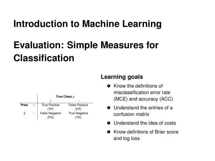
Introduction to Machine Learning Evaluation: Simple Measures for Classification

Learning goals

Know the definitions of misclassification error rate (MCE) and accuracy (ACC) Understand the entries of a confusion matrix Understand the idea of costs Know defintions of Brier score and log loss

LABELS VS PROBABILITIES

In classification we predict:

1

Class labels → ˆ h(x) = ˆ y

2

Class probabilities → ˆ

πk(x) → We evaluate based on those

c

• Introduction to Machine Learning – 1 / 9

LABELS: MCE

The misclassification error rate (MCE) counts the number of incorrect predictions and presents them as a rate: MCE = 1 n

n

• i=1

[y(i) = ˆ

y(i)] ∈ [0; 1] Accuracy is defined in a similar fashion for correct classifications: ACC = 1 n

n

• i=1

[y(i) = ˆ

y(i)] ∈ [0; 1] If the data set is small this can be brittle The MCE says nothing about how good/skewed predicted probabilities are Errors on all classes are weighed equally (often inappropriate)

c

• Introduction to Machine Learning – 2 / 9

LABELS: CONFUSION MATRIX

True classes in columns. Predicted classes in rows.

setosa versicolor virginica -err.- -n- setosa 50 50 versicolor 46 4 4 50 virginica 4 46 4 50

• err.-

4 4 8 NA

• n-

50 50 50 NA 150

We can see class sizes (predicted and true) and where errors occur.

c

• Introduction to Machine Learning – 3 / 9

LABELS: CONFUSION MATRIX

In binary classification

True Class y

+ −

Pred.

+

True Positive (TP) False Positive (FP)

ˆ

y

−

False Negative (FN) True Negative (TN)

c

• Introduction to Machine Learning – 4 / 9

LABELS: COSTS

We can also assign different costs to different errors via a cost matrix. Costs = 1 n

n

• i=1

C[y(i), ˆ y(i)] Example: Predict if person has a ticket (yes / no). Should train conductor check ticket of a person? Costs: Ticket checking: 3 EUR Fee for fare-dodging: 40 EUR

http: //www.oslobilder.no/OMU/OB.%C3%9864/2902 c

• Introduction to Machine Learning – 5 / 9

LABELS: COSTS

Predict if person has a ticket (yes / no).

Cost matrix C predicted true no yes no

• 37

yes 3 Confusion matrix predicted true no yes no 7 yes 93 Confusion matrix * C predicted true no yes no

• 259

yes 279

Costs: Ticket checking: 3 EUR Fee for fare-dodging: 40 EUR Our model says that we should not trust anyone and check the tickets of all passengers. Costs = 1 n

n

• i=1

C[y(i), ˆ y(i)]

=

1 100 (−37 · 7 + 0 · 0 + 3 · 93 + 0 · 0)

= 20

100 = 0.2

c

• Introduction to Machine Learning – 6 / 9

PROBABILITIES: BRIER SCORE

Measures squared distances of probabilities from the true class labels: BS1 = 1 n

n

• i=1
• ˆ

π(x(i)) − y(i)2

Fancy name for MSE on probabilities Usual definition for binary case, y(i) must be coded as 0 and 1.

right wrong wrong right

0.00 0.25 0.50 0.75 1.00 0.00 0.25 0.50 0.75 1.00

π ^(x) BS true.label

1 c

• Introduction to Machine Learning – 7 / 9

PROBABILITIES: BRIER SCORE

BS2 = 1 n

n

• i=1

g

• k=1
• ˆ

πk(x(i)) − o(i)

k

2

Original by Brier, works also for multiple classes

• (i)

k

= [y(i) = k] is a 0-1-one-hot coding for labels

For the binary case, BS2 is twice as large as BS1, because in BS2 we sum the squared difference for each observation regarding class 0 and class 1, not only the true class.

c

• Introduction to Machine Learning – 8 / 9

PROBABILITIES: LOG-LOSS

Logistic regression loss function, a.k.a. Bernoulli or binomial loss, y(i) coded as 0 and 1. LL = 1 n

n

• i=1
• −y(i) log(ˆ

π(x(i))) − (1 − y(i)) log(1 − ˆ π(x(i)))

• right

wrong wrong right

1 2 3 4 0.00 0.25 0.50 0.75 1.00

π ^(x) LL true.label

1

Optimal value is 0, “confidently wrong” is penalized heavily Multiclass version: LL = − 1

n n

• i=1

g

• k=1
• (i)

k log(ˆ

πk(x(i)))

c

• Introduction to Machine Learning – 9 / 9