introduction to graphs
play

Introduction to Graphs V = nodes. E = edges between pairs of nodes. - PowerPoint PPT Presentation

Undirected graphs Notation. G = ( V , E ) Introduction to Graphs V = nodes. E = edges between pairs of nodes. Captures pairwise relationship between objects. Tyler Moore Graph size parameters: n = | V |, m = | E | . CS 2123, The


  1. Undirected graphs Notation. G = ( V , E ) Introduction to Graphs ・ V = nodes. ・ E = edges between pairs of nodes. ・ Captures pairwise relationship between objects. Tyler Moore ・ Graph size parameters: n = | V |, m = | E | . CS 2123, The University of Tulsa V = { 1, 2, 3, 4, 5, 6, 7, 8 } E = { 1-2, 1-3, 2-3, 2-4, 2-5, 3-5, 3-7, 3-8, 4-5, 5-6, 7-8 } Some slides created by or adapted from Dr. Kevin Wayne. For more information see http://www.cs.princeton.edu/~wayne/kleinberg-tardos m = 11, n = 8 3 2 / 36 One week of Enron emails The evolution of FCC lobbying coalitions “The Evolution of FCC Lobbying Coalitions” by Pierre de Vries in JoSS Visualization Symposium 2010 4 5 3 / 36 4 / 36

  2. Social Network as a Graph Framingham heart study Nodes: people Alice Edges: friendship Bob Charlie Dawn Eve Figure 1. Largest Connected Subcomponent of the Social N etwork in the Framingham H eart Study in the Year 2000. Each circle (node) represents one person in the data set. There are 2200 persons in this subcomponent of the social George Fred network. Circles with red borders denote women, and circles with blue borders denote men. The size of each circle is proportional to the person’s body-mass index. The interior color of the circles indicates the person’s obesity status: yellow denotes an obese person (body-mass index, ≥ 30) and green denotes a nonobese person. The colors of the ties between the nodes indicate the relationship between them: purple denotes a friendship or marital tie and orange denotes a familial tie. “The Spread of Obesity in a Large Social Network over 32 Years” by Christakis and Fowler in New England Journal of Medicine, 2007 6 5 / 36 6 / 36 Road Network as a Graph Electronic Circuits as a Graph 10Ω Nodes: intersections A Main St Edges: roads v x S 20Ω 5Ω 5 v x 2nd Ave 1st Ave M B 3rd Ave t S a i m n S l E t Aspen Ave M t 5th Ave S a k i n Vertices: junctions r a S P t Edges: components 5th Ave 7 / 36 8 / 36

  3. Course Dependencies as a Graph Maze as a Graph CS 1043 CS 2003 CS 2033 CS 2123 Nodes: courses Edges: prerequisites CS 3053 Nodes: rooms; edges: doorways CS 4333 10 / 36 11 / 36 Flavors of Graphs Directed vs. Undirected Graphs A Undirected A Directed B C B C The first step in any graph problem is recognizing that you have a graph problem D E D E It’s not always obvious! The second step in any graph problem is determining which flavor of F G F G graph you are dealing with Learning to talk the talk is an important part of walking the walk A graph G = ( V , E ) is undirected if edge ( x , y ) ∈ E implies that The flavor of graph has a big impact on which algorithms are ( y , x ) is also in E appropriate and efficient Road networks between cities are typically undirected Street networks within cities are almost always directed because of one-way streets What about online social networks? 12 / 36 13 / 36

  4. Exercise 1: Spot the graph Exercise 2: Spot the graph Pay From Pay To Amount Date 12354 67324 $1000 Sep 1 12398 67324 $500 Sep 4 67324 45721 $750 Sep 7 78923 12398 $500 Sep 8 Nodes: Edges: Nodes: Edges: 14 / 36 15 / 36 Exercise 3: Spot the graph Exercise 4: Spot the graph def foo(arg1): x = arg1+2 x = [’ham’,’spam’,’glam’,’tram’] bar(x) for a in x: print a def bar(arg1,arg2): if a ==’ham’: y = arg1+arg2 print ’awesome’ ham(y) else: print ’terrible’ print ’moving on’ def ham(arg1): bar(2*arg1) Nodes: Edges: Nodes: Edges: 16 / 36 17 / 36

  5. Some graph applications
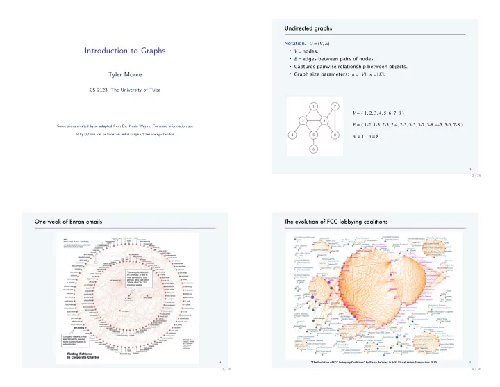
 Some directed graph applications directed graph node directed edge graph node edge transportation street intersection one-way street communication telephone, computer fiber optic cable web web page hyperlink circuit gate, register, processor wire food web species predator-prey relationship mechanical joint rod, beam, spring WordNet synset hypernym financial stock, currency transactions scheduling task precedence constraint transportation street intersection, airport highway, airway route financial bank transaction internet class C network connection cell phone person placed call infectious disease person infection game board position legal move game board position legal move social relationship person, actor friendship, movie cast citation journal article citation neural network neuron synapse object graph object pointer protein network protein protein-protein interaction inheritance hierarchy class inherits from molecule atom bond control flow code block jump 7 39 18 / 36 19 / 36 Weighted vs. Unweighted Graphs Cyclic vs. Acyclic Graphs Unweighted Weighted A A Cyclic Acyclic A A 10 4 B C B C 1 B C B C 7 5 8 19 D E D E D D 4 0 6 1 8 F G F G F G F G In weighted graphs, each edge (or vertex) of G is assigned a An acyclic graph does not contain any cycles numerical value, or weight Trees are connected, acyclic, undirected graphs The edges of a road network graph might be weighted with their Directed acyclic graphs are called DAGs length, drive-time or speed limit DAGs arise naturally in scheduling problems, where a directed edge In unweighted graphs, there is no cost distinction between various ( x , y ) indicates that x must occur before y . edges and vertices 20 / 36 21 / 36

  6. Labeled vs. Unlabeled Graphs More Graph Terminology Labeled Unlabeled A B C A path is a sequence of edges connecting two vertices Two common problems: (1) does a path exist between A and B ? (2) D E what is the shortest path between A and B ? A graph is connected if there is a path between any two vertices F G A directed graph is strongly connected if there is a directed path between any two vertices. In labeled graphs, each vertex is assigned a unique name or identifier The degree of a vertex is the number of edges adjacent to it to distinguish it from all other vertices. An important graph problem is isomorphism testing: determining whether the topological structure of two graphs are in fact identical if we ignore any labels. 22 / 36 23 / 36 Graph representation: adjacency matrix Graph representation: adjacency lists Adjacency matrix. n -by- n matrix with A uv = 1 if ( u , v ) is an edge. Adjacency lists. Node indexed array of lists. ・ Two representations of each edge. ・ Two representations of each edge. degree = number of neighbors of u ・ Space proportional to n 2 . ・ Space is Θ ( m + n ) . ・ Checking if ( u , v ) is an edge takes Θ (1) time. ・ Checking if ( u , v ) is an edge takes O ( degree ( u )) time. ・ Identifying all edges takes Θ ( n 2 ) time. ・ Identifying all edges takes Θ ( m + n ) time. 1 2 3 1 2 3 4 5 6 7 8 2 1 3 4 5 1 0 1 1 0 0 0 0 0 2 1 0 1 1 1 0 0 0 1 2 5 7 8 3 3 1 1 0 0 1 0 1 1 4 2 5 4 0 1 0 0 1 0 0 0 5 2 3 4 6 5 0 1 1 1 0 1 0 0 6 0 0 0 0 1 0 0 0 6 5 7 0 0 1 0 0 0 0 1 7 3 8 8 0 0 1 0 0 0 1 0 8 3 7 8 9 24 / 36 25 / 36

  7. Graph Data Structures Graph Data Structures Option 1: Adjacency Sets Option 2: Adjacency Lists a , b , c , d , e , f , g , h = range (8) a , b , c , d , e , f , g , h = range (8) N = [ N = [ { b , c , d , e , f } , # a [ b , c , d , e , f ] , # a { c , e } , # b [ c , e ] , # b { d } , # c [ d ] , # c g g c c b b { e } , # d [ e ] , # d { f } , # e [ f ] , # e { c , g , h } , # f [ c , g , h ] , # f { f , h } , # g [ f , h ] , # g a a f { f , g } # h f [ f , g ] # h ] ] > b i n N[ a ] > b i n N[ a ] > > > > e e d h d h # Neighborhood membership # Neighborhood membership True True > len (N[ f ] ) # Degree > len (N[ f ] ) # Degree > > > > 3 3 26 / 36 26 / 36 Graph Data Structures Graph Data Structures Option 3: Adjacency Dictionaries w/ Edge Weights Option 4: Dictionaries w/ Adjacency Sets a , b , c , d , e , f , g , h = range (8) N = [ N = { { b : 2 , c : 1 , d : 3 , e : 9 , f :4 } , #a ’ a ’ : set ( ’ bcdef ’ ) , { c : 4 , e : 3 } , #b ’ b ’ : set ( ’ ce ’ ) , { d : 8 } , #c ’ c ’ : set ( ’ d ’ ) , { e : 7 } , #d g c 4 b g c ’ d ’ : set ( ’ e ’ ) , b { f : 5 } , #e ’ e ’ : set ( ’ f ’ ) , 2 { c : 2 , g : 2 , h : 2 } , #f 1 ’ f ’ : set ( ’ cgh ’ ) , 2 2 { f : 1 , h : 6 } , #g 1 ’ g ’ : set ( ’ fh ’ ) , { f : 9 , g :8 } #h a 4 f ’ h ’ : set ( ’ fg ’ ) a 8 3 f ] 8 6 } 2 9 3 5 > b i n N[ a ] 9 > > > ’ b ’ i n N[ ’ a ’ ] > > # Neighborhood membership e 7 d h # Neighborhood membership e d h True True > len (N[ f ] ) # Degree > > > len (N[ ’ f ’ ] ) # Degree > > 3 3 > N[ a ] [ b ] > > # Edge weight f o r ( a , b ) 2 26 / 36 26 / 36

Download Presentation
Download Policy: The content available on the website is offered to you 'AS IS' for your personal information and use only. It cannot be commercialized, licensed, or distributed on other websites without prior consent from the author. To download a presentation, simply click this link. If you encounter any difficulties during the download process, it's possible that the publisher has removed the file from their server.

Recommend


More recommend