Introduction to advanced parameter Gradient descent algorithm - - PowerPoint PPT Presentation

Introduction to advanced parameter

• ptimization

So far:

• What is a neural network?
• Basic training algorithm:
• Gradient descent
• Backpropagation

Next: advanced training algorithms

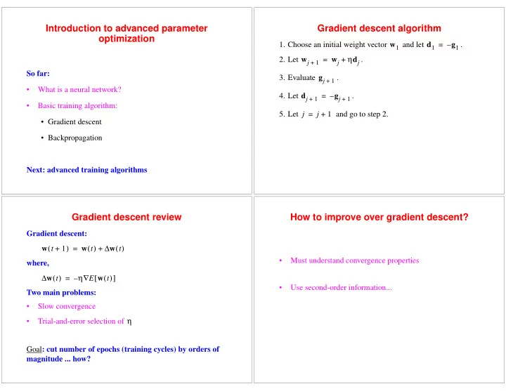
Gradient descent algorithm

• 1. Choose an initial weight vector

and let .

• 2. Let

.

• 3. Evaluate

.

• 4. Let

.

• 5. Let

and go to step 2. w1 d1 g1 – = wj

1 +

wj ηdj + = gj

1 +

dj

1 +

gj

1 +

– = j j 1 + =

Gradient descent review

Gradient descent: where, Two main problems:

• Slow convergence
• Trial-and-error selection of

Goal : cut number of epochs (training cycles) by orders of magnitude ... how? w t 1 + ( ) w t ( ) w t ( ) ∆ + = w t ( ) ∆ η E w t ( ) [ ] ∇ – = η

How to improve over gradient descent?

• Must understand convergence properties
• Use second-order information...

First case study

(same as last time) Will also look at simple nonquadratic error surfaces... E 20ω1

2

ω2

2

+ =

• 1.5
• 1
• 0.5

0.5 1

• 0.5

0.5 1 1.5 2 20 40 1.5

• 1
• 0.5

0.5

ω1 ω2 E

Why quadratic error surface?

Disadvantages:

• Too simple/too few parameters
• NN error surface not

globally quadratic Advantage:

• Easy to visualize
• NN error surfaces will be

locally quadratic near a local minimum.

Taylor series expansion

Single dimension (from calculus): Multi-dimensional error surface: about some vector , where, ( Hessian: not just a German mercenary) f x ( ) f x0 ( ) f' x0 ( ) x x0 – ( ) f'' x0 ( ) x x0 – ( )2 + + ≈ E w ( ) E w0 ( ) w w0 – ( )Tb 1 2

• w

w0 – ( )TH w w0 – ( ) + + ≈ w0 b E w0 ( ) ∇ = H E w0 ( ) ∇ [ ] ∇ =

Hessian matrix

Definition: The Hessian matrix

• f a
• dimensional function

is defined as, where, Alternatively: W W × H W E w ( ) H E w ( ) ∇ [ ] ∇ = w ω1 ω2 … ωW

T

= H i j

, ( )

∂2E ∂ωi∂ωj

• =

Some linear algebra

Definition: For a square matrix , the eigenvalues are the solution of, Definition: A square matrix is positive-definite, if and

• nly if all its eigenvalues

are greater than zero. If a matrix is positive-definite, then, , .

• Quadratic error surface:
• Arbitrary error surface:

near local minimum. W W × H λ λIW H – = H λi vTHv > v ∀ ≠ H > H >

Gradient descent convergence rate

Near local minimum: (why?) Convergence governed by: Learning rate bound: λmin > λmin λmax

• 

   η 2 λmax

• <

<

Simple Hessian example

First partial derivatives: Second partial derivatives: E 20ω1

2

ω2

2

+ = E ∂ ω1 ∂

• 40ω1

= E ∂ ω2 ∂

• 2ω2

= ∂2E ∂ω1

2

• 40

= ∂2E ∂ω2

2

• 2

= ∂2E ∂ω1∂ω2

• ∂2E

∂ω2∂ω1

• =

=

Simple Hessian example (continued)

Second partial derivatives: Hessian: E 20ω1

2

ω2

2

+ = ∂2E ∂ω1

2

• 40

= ∂2E ∂ω2

2

• 2

= ∂2E ∂ω1∂ω2

• ∂2E

∂ω2∂ω1

• =

= H 40 0 0 2 =

Simple Hessian example (continued)

What are the eigenvalues? H 40 0 0 2 =

Computation of eigenvalues

λI2 H – = λ 1 0 0 1 40 0 0 2 – = λ 40 – λ 2 – = λ 40 – ( ) λ 2 – ( ) = λmin 2 = λmax 40 =

Learning rate bounds

(same as fixed-point derivation) λmin 2 = λmax 40 = η 2 λmax

• <

< η 2 40

• <

< 0.05 =

Convergence examples

• 1.5
• 1
• 0.5

0.5 1

• 0.5

0.5 1 1.5 2

ω1 ω2 η 0.01 = 719 steps

Convergence examples

• 1.5
• 1
• 0.5

0.5 1

• 0.5

0.5 1 1.5 2

ω2 ω1 η 0.04 = 175 steps

Convergence examples

• 1.5
• 1
• 0.5

0.5 1

• 0.5

0.5 1 1.5 2

ω1 η 0.05 = no convergence

Basic problem: “long valley with steep sides”

What characterizes a “ long valley with steep sides?” Length of contour lines proportional to: and Small ratios: So what can we do about this? 1 λ1

• 1

λ2

• λmin

λmax

• 

  

Solution

• Fixed learning rate is the problem
• Answer: different learning rates for each weight.

Key question: how to achieve automatically?

Heuristic extension: momentum

Gradient descent with momentum: , , Notes:

• dependent on

and

• Ideally, high effective learning rate in shallow dimensions
• Little effect along steep dimensions

µ w t 1 + ( ) w t ( ) w t ( ) ∆ + = w 0 ( ) ∆ η E w 0 ( ) [ ] ∇ – = w t ( ) ∆ η E w t ( ) [ ] ∇ – µ∆w t 1 – ( ) + = t > µ ≤ 1 < w t ( ) ∆ w t ( ) w t 1 – ( )

Gradient descent algorithm

• 1. Choose an initial weight vector

and let .

• 2. Let

.

• 3. Evaluate

.

• 4. Let

.

• 5. Let

and go to step 2. w1 d1 g1 – = wj

1 +

wj ηdj + = gj

1 +

dj

1 +

gj

1 +

– = j j 1 + =

Analyzing momentum term

Shallow regions: assume, , Then: E wt ( ) ∇ E w0 ( ) ∇ ≈ g = t 1 2 … , , { } ∈ w 0 ( ) ∆ ηg – = w 1 ( ) ∆ ηg – µ w 0 ( ) ∆ + ≈ ηg 1 µ + ( ) – = w 2 ( ) ∆ ηg – µ w 1 ( ) ∆ + ≈ ηg – µ ηg 1 µ + ( ) – [ ] + = w 2 ( ) ∆ ηg 1 µ µ2 + + ( ) – ≈

Analyzing momentum term

Assumption (shallow region): , In general, In the limit: E wt ( ) ∇ E w0 ( ) ∇ ≈ g = t 1 2 … , , { } ∈ w t ( ) ∆ ηg µs

s = t

∑

      – ≈ η 1 µt

1 +

– 1 µ –

• 

   g – = w t ( ) ∆ η – 1 µ – ( )

• g

≈

t ∞ →

lim

Analyzing momentum term

Effective learning rate (shallow regions): η 1 µ – ( ) ⁄

Analyzing momentum term

Steep regions: oscillations Net effect (ideally): little E w t 1 + ( ) [ ] ∇ E w t ( ) [ ] ∇ – ≈

Momentum

Advantage:

• Increase effective learning rate in shallow regions

Disadvantages:

• Yet another parameter to hand tune
• If not carefully chosen,

can do more harm than good µ

Convergence examples

• 1.5
• 1
• 0.5

0.5 1

• 0.5

0.5 1 1.5 2

ω1 ω2 η 0.01 µ , 0.0 = =

719 steps

Convergence examples

• 1.5
• 1
• 0.5

0.5 1

• 0.5

0.5 1 1.5 2

ω1 ω2 η 0.01 µ , 0.5 = =

341 steps

Convergence examples

• 1.5
• 1
• 0.5

0.5 1

• 0.5

0.5 1 1.5 2

ω1 ω2 η 0.01 µ , 0.9 = =

266 steps

Convergence examples

• 1.5
• 1
• 0.5

0.5 1

• 0.5

0.5 1 1.5 2

ω2 ω1 η 0.04 µ , 0.0 = =

175 steps

Convergence examples

• 1.5
• 1
• 0.5

0.5 1

• 0.5

0.5 1 1.5 2

ω2 ω1 η 0.04 µ , 0.5 = =

60 steps

Convergence examples

• 1.5
• 1
• 0.5

0.5 1

• 1
• 0.5

0.5 1 1.5 2

ω2 ω1 η 0.04 µ , 0.9 = =

272 steps

Convergence examples: summary

719 341 266 175 60 272 µ 0.0 = µ 0.5 = µ 0.9 = η 0.01 = η 0.04 =

Heuristic extensions to gradient descent

Momentum popular in neural network community. Many other heuristic attempts (some examples):

• Adaptive learning rate (what should

and be?)

• (what’s the problem here?)

ρ σ ηnew ρηold E ∆ < σηold E ∆ >    = ηmax 2 λmax ⁄ =

Heuristic extensions to gradient descent

• Individual learning rates:

(problems?)

• Quickprop: local independent quadratic assumption:

(problems?) ηi ∆ γgi

t ( )gi t 1 – ( )

= ωi ∆

t 1 + ( )

gi

t ( )

gi

t 1 – ( )

gi

t ( )

–

• ωi

∆

t ( )

=

Heuristic extensions to gradient descent

Problems:

• Additional hand-tuned parameters
• Independence of weight assumptions

More principled approach is desirable.

Steepest descent

Gradient descent: where, Question: why take all those little tiny steps? w t 1 + ( ) w t ( ) w t ( ) ∆ + = w t ( ) ∆ η E w t ( ) [ ] ∇ – =

Steepest descent: gradient descent with line minimization

• 1. Define search direction

:

• 2. Minimize:

such that: ,

• 3. New update:

(problems?) d t ( ) d t ( ) E w t ( ) [ ] ∇ – = E η ( ) E w t ( ) ηd t ( ) + [ ] ≡ E η∗ ( ) E η ( ) ≤ η ∀ w t 1 + ( ) w t ( ) η∗d t ( ) + =

Steepest descent

Question: Do we need to compute ? Answer: No. Use one-dimensional line search, which requires only evaluation of . Line search: two steps

• 1. Bracket minimum
• 2. Line minimization

∂E ∂η ⁄ E η ( )

Line search: bracketing the minimum

Basic problem: need three values such that: a b c , , E a ( ) E b ( ) > E c ( ) E b ( ) >

1 2 3 4 5 6 7 8 1 2 3 4 5 6

η E η ( ) a b c

Bracketing the minimum

• 1. Let

. Let . Note: will satisfy (why?).

• 2. Let

, where (what should be?).

• 3. If

, then done; else, let and . Repeat step 2. Note: one evaluation of per step. a = b ε = E a ( ) E b ( ) > c k b a – ( ) a + = k 1 > k E c ( ) E b ( ) > a b = b c = E

Bracketing example

1 2 3 4 5 6 7 8 1 2 3 4 5 6 1 2 3 4 5 6 7 8 1 2 3 4 5 6 1 2 3 4 5 6 7 8 1 2 3 4 5 6 1 2 3 4 5 6 7 8 1 2 3 4 5 6

η η η η E η ( ) E η ( ) E η ( ) E η ( )

#1 #2 #3 #4

Bracketing example: error surface

E ω1 ω2 , ( ) 1 5ω1

2

– ω2

2

– ( ) exp – =

• 2
• 1

1 2

• 2
• 1

1 2 0.25 0.5 0.75 1

• 2
• 1

1

ω2 ω1

What is ?

Weights At : E η ( ) ω1 ω2 , ( ) 1 2 , ( ) = E ω1 ω2 , ( ) ∇ 10ω1 5ω1

2

– ω2

2

– ( ) exp 2ω2 , [ ] 5ω1

2

– ω2

2

– ( ) exp = E η ( ) 1 5 ω1 10ω1η 5ω1

2

– ω2

2

– ( ) exp – ( )2 – – ( exp – = ω2 2ω2η 5ω1

2

– ω2

2

– ( ) exp – ( )2) ω1 ω2 , ( ) 1 2 , ( ) = E η ( ) 1 5 1 10η 9 – ( ) exp – ( )2 – 2 4η 9 – ( ) exp – ( )2 – ( ) exp – =

Bracketing example: error surface

200 400 600 800 1000 1200 1400 0.92 0.94 0.96 0.98 1

η E η ( ) a b c

Line minimization

• 1. Pick a value of

in larger interval:

• r

.

• 2. If

is larger interval, set new bracketing values to: if , (set ), or , if , (set and ). Else, set new bracketing values to, if , (set ), or , if , (set and ).

• 3. Iterate steps 1 and 2 until

. η x = a b , ( ) b c , ( ) a b , ( ) x b c , , { } E x ( ) E b ( ) > a x = a x b , , { } E b ( ) E x ( ) > c b = b x = a b x , , { } E x ( ) E b ( ) > c x = b x c , , { } E b ( ) E x ( ) > a b = b x = c a – ( ) θ <

Line minimization

What should the value of be? [ is larger interval] [ is larger interval] Rate of convergence proportional to: (golden mean) x x 0.381966 c b – ( ) b + = b c , ( ) x b 0.381966 b a – ( ) – = a b , ( ) 1 k

• 0.61803

≈ k 1 5 + 2

• 1.61803

≈ =

Examples: quadratic surface

• 1
• 0.5

0.5 1 0.5 1 1.5 2

ω2 ω1 steepest descent 15 steps to convergence

Examples: quadratic surface (comparison)

• 1
• 0.5

0.5 1 0.5 1 1.5 2

ω2 ω1 η 0.04 = ( ) gradient descent 175 steps to convergence

Examples: nonquadratic surface

• 1
• 0.5

0.5 1 0.5 1 1.5 2

ω2 ω1 steepest descent 24 steps to convergence

Examples: nonquadratic surface

• 1
• 0.5

0.5 1 1.5

• 1.5
• 1
• 0.5

0.5 1 1.5 2

ω2 ω1 η 0.2 = ( ) gradient descent 456 steps to convergence

Computational complexity

Steepest descent: computations/step (why?) Gradient descent: computations/step 5NW 10 2NW ( ) + 25NW = 5NW

Discussion

What’s bad about steepest descent? Answer: Orthogonality of consecutive steps.

• Why does this occur?
• Can we do better?