Conjugate gradient training algorithm Steepest descent algorithm - - PowerPoint PPT Presentation

SLIDE 1

Conjugate gradient training algorithm

So far:

• Heuristic improvements to gradient descent (momentum)
• Steepest descent training algorithm
• Can we do better?

Next: Conjugate gradient training algorithm

• Overview
• Derivation
• Examples

Steepest descent algorithm

Definitions:

• = weight vector at step .
• = gradient at step .
• = search direction at step .

wj j gj E wj [ ] ∇ = j dj j

Steepest descent algorithm

• 1. Choose an initial weight vector

and let .

• 2. Perform line minimization along

, , such that: , .

• 3. Let

.

• 4. Evaluate

.

• 5. Let

.

• 6. Let

and go to step 2. w1 d1 g1 – = dj j 1 ≥ E wj η∗dj + ( ) E wj ηdj + ( ) ≤ η ∀ wj

1 +

wj η∗dj + = gj

1 +

dj

1 +

gj

1 +

– = j j 1 + =

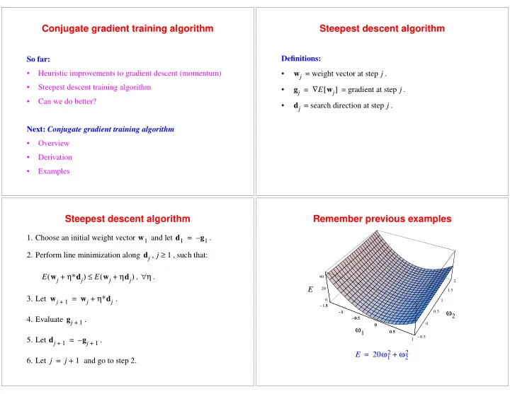
Remember previous examples

• 1.5
• 1
• 0.5

0.5 1

• 0.5

0.5 1 1.5 2 20 40 1.5

• 1
• 0.5

0.5

ω1 ω2 E E 20ω1

2

ω2

2

+ =

SLIDE 2

Remember previous examples

• 2
• 1

1 2

• 2
• 1

1 2 0.25 0.5 0.75 1

• 2
• 1

1

ω2 ω1 E ω1 ω2 , ( ) 1 5ω1

2

– ω2

2

– ( ) exp – =

Steepest descent algorithm examples

• 1
• 0.5

0.5 1 0.5 1 1.5 2

ω2 ω1

steepest descent 15 steps to convergence

• 1
• 0.5

0.5 1 0.5 1 1.5 2

ω2 ω1

steepest descent 24 steps to convergence

quadratic non-quadratic

Conjugate gradient algorithm (a sneak peek)

• 1. Choose an initial weight vector

and let .

• 2. Perform a line minimization along

, such that: , .

• 3. Let

.

• 4. Evaluate

.

• 5. Let

where,

• 6. Let

and go to step 2. w1 d1 g1 – = dj E wj η∗dj + ( ) E wj ηdj + ( ) ≤ η ∀ wj

1 +

wj η∗dj + = gj

1 +

dj

1 +

gj

1 +

– βjdj + = βj gj

1 + T

gj

1 +

gj – ( ) gj

Tgj

• =

j j 1 + =

Conjugate gradient algorithm (sneak peak)

quadratic non-quadratic

• 1
• 0.5

0.5 1 0.5 1 1.5 2

ω1 ω2

conjugate gradient 5 steps to convergence

• 1
• 0.5

0.5 1 0.5 1 1.5 2

ω1 ω2

conjugate gradient 2 steps to convergence

SLIDE 3

SD vs. CG

Key difference: new search direction

• Very little additional computation (over steepest descent).
• No more oscillation back and forth.

Key question:

• Why/How does this improve things?

Knowledge of local quadratic properties of error surface...

Conjugate gradients: a first look

In steepest descent: (What does this mean?) g w t 1 + ( ) [ ]Td t ( ) =

Conjugate gradients: a first look

Non-interfering directions: , (What the #$@!# does this mean?) g w t 1 + ( ) ηd t 1 + ( ) + [ ]Td t ( ) = η ≥

How do we achieve non-interfering directions?

FACT: , implies (H-orthogonality, conjugacy) Hmmm ... need to pay attention to 2nd-order properties of error surface... g w t 1 + ( ) ηd t 1 + ( ) + [ ]Td t ( ) = η ≥ d t 1 + ( )THd t ( ) = E w ( ) E0 bTw 1 2

• wTHw

+ + =

SLIDE 4

Show H-orthogonality requirement

Approximate by 1st-order Taylor approximation about : Let : Evaluate at : g w ( ) w0 g w ( )T g w0 ( )T w w0 – ( )T g w0 ( ) { } ∇ + ≈ w0 w t 1 + ( ) = g w ( )T g w t 1 + ( ) [ ]T w w t 1 + ( ) – [ ]T g w t 1 + ( ) [ ] { } ∇ + = g w ( ) w w t 1 + ( ) ηd t 1 + ( ) + = g w t 1 + ( ) ηd t 1 + ( ) + [ ]T g w t 1 + ( ) [ ]T ηd t 1 + ( )TH + =

Show H-orthogonality requirement

Post-multiply by :

• Left-hand side:

(assumption)

• Right-hand side:

(implication) g w t 1 + ( ) ηd t 1 + ( ) + [ ]T g w t 1 + ( ) [ ]T ηd t 1 + ( )TH + = d t ( ) g w t 1 + ( ) ηd t 1 + ( ) + [ ]Td t ( ) = g w t 1 + ( ) [ ]Td t ( ) ηd t 1 + ( )THd t ( ) + = ηd t 1 + ( )THd t ( ) = d t 1 + ( )THd t ( ) =

How do we achieve non-interfering directions?

Proven fact: , implies (H-orthogonality) Key: need to construct consecutive search directions that are conjugate (

• orthogonal)!

(Side note: What is the implicit assumption of SD?) g w t 1 + ( ) ηd t 1 + ( ) + [ ]Td t ( ) = η ≥ d t 1 + ( )THd t ( ) = d H

Derivation of conjugate gradient algorithm

• Local quadratic assumption:
• Assume:
• mutually conjugate vectors

.

• Initial weight vector

. Question: How to converge to in (at most) steps? E w ( ) E0 bTw 1 2

• wTHw

+ + = W di w1 w∗ W

SLIDE 5

Step-wise optimization

(why can I do this?) w∗ w1 – ( ) αidi

i 1 = W

∑

= w∗ w1 αidi

i 1 = W

∑

+ = wj w1 αidi

i 1 = j 1 –

∑

+ ≡ wj

1 +

wj αjdj + =

Linear independence of conjugate directions

Theorem: For a positive-definite square matrix ,

• rthogonal vectors

are linearly independent. Proof: Linear independence: iff. , . H H d1 d2 … dk , , , { } α1d1 α2d2 … αkdk + + + = αi = i ∀

Linear independence of conjugate directions

Linear independence: iff. , . Pre-multiply by : Note (by assumption): , . α1d1 α2d2 … αkdk + + + = αi = i ∀ di

TH

α1di

THd1

α2di

THd2

… αkdi

THdk

+ + + di

TH0

= α1di

THd1

α2di

THd2

… αkdi

THdk

+ + + = di

THdj

= i ∀ j ≠

Linear independence of conjugate directions

reduces to: However: (by assumption) Therefore: , ❏ α1di

THd1

α2di

THd2

… αkdi

THdk

+ + + = αidi

THdi

= di

THdi

> αi = i 1 2 … k , , , { } ∈

SLIDE 6

Linear independence of conjugate directions

From linear independence:

• orthogonal vectors

form a complete basis set.

• Any vector

can be expressed as: So, why did we need this result? H di v v αidi

i 1 = W

∑

=

Step-wise optimization

(Ah-ha!) w∗ w1 – ( ) αidi

i 1 = W

∑

= w∗ w1 αidi

i 1 = W

∑

+ = wj w1 αidi

i 1 = j 1 –

∑

+ ≡ wj

1 +

wj αjdj + =

So where are we now?

On locally quadratic surface, can converge to minimum in, at most, steps using: , . Big Questions:

• How to choose step size

?

• How to construct conjugate directions

?

• How can we do everything without computing

? W wj

1 +

wj αjdj + = j 1 2 … W , , , { } = αj dj H

Computing the correct step size

Given: a set of conjugate vectors . Pre-multiply by : αj W di w∗ w1 – ( ) αidi

i 1 = W

∑

= dj

TH

dj

TH w∗

w1 – ( ) dj

TH

αidi

i 1 = W

∑

      = dj

TH w∗

w1 – ( ) αidj

THdi i 1 = W

∑

=

SLIDE 7

Computing the correct step size

By

• orthogonality (conjugacy assumed):

(why?) αj dj

TH w∗

w1 – ( ) αidj

THdi i 1 = W

∑

= H dj

TH w∗

w1 – ( ) αjdj

THdj

=

Computing the correct step size

Also: At minimum: αj E w ( ) E0 bTw 1 2

• wTHw

+ + = g w ( ) b Hw + = g w∗ ( ) = b Hw∗ + = Hw∗ b – =

Computing the correct step size

So: (what’s the problem?) αj dj

TH w∗

w1 – ( ) αjdj

THdj

= Hw∗ b – = dj

T

b – Hw1 – ( ) αjdj

THdj

= dj

T b

Hw1 + ( ) – αjdj

THdj

= αj dj

T b

Hw1 + ( ) – dj

THdj

• =

Computing the correct step size

Pre-multiply by : . . αj αj dj

T b

Hw1 + ( ) – dj

THdj

• =

wj w1 αidi

i 1 = j 1 –

∑

+ = dj

TH

dj

THwj

dj

THw1

αidj

THdi i 1 = j 1 –

∑

+ = dj

THwj

dj

THw1

= αj dj

T b

Hwj + ( ) – dj

THdj

• =

SLIDE 8

Computing the correct step size

So: (woo-hoo!) αj αj dj

T b

Hwj + ( ) – dj

THdj

• =

gj b Hwj + = αj dj

Tgj

– dj

THdj

• =

Important consequence

Theorem: Assuming a

• dimensional quadratic error

surface, and

• orthogonal vectors

, : will converge in at most steps to the minimum (for what error surface?). W E w ( ) E0 bTw 1 2

• wTHw

+ + = H di i 1 2 … W , , , { } ∈ wj

1 +

wj αjdj + = αj dj

Tgj

– dj

THdj

• =

W w∗

Why is this so?

FACT: , How is this important? How is this different from steepest descent? Let’s show that this is true... dk

Tgj

= k ∀ j <

Orthogonality of gradient to previous search directions

So: gj b Hwj + = wj

1 +

wj αjdj + = gj

1 +

gj – H wj

1 +

wj – ( ) = wj

1 +

wj – ( ) αjdj = gj

1 +

gj – αjHdj =

SLIDE 9

Orthogonality of gradient to previous search directions

Pre-multiply by : gj

1 +

gj – αjHdj = αj dj

Tgj

– dj

THdj

• =

dj

T

dj

T gj 1 +

gj – ( ) αjdj

THdj

= dj

T gj 1 +

gj – ( ) dj

Tgj

– dj

THdj

• 

     dj

THdj

=

Orthogonality of gradient to previous search directions

So: , (need to show for all ) dj

T gj 1 +

gj – ( ) dj

Tgj

– dj

THdj

• 

     dj

THdj

= dj

T gj 1 +

gj – ( ) dj

Tgj

– = dj

Tgj 1 +

dj

Tgj

– dj

Tgj

– = dj

Tgj 1 +

= dk

Tgj

= k j 1 – = k j <

Orthogonality of gradient to previous search directions

Pre-multiply by : . (why?) , gj

1 +

gj – αjHdj = dk

T

dk

T gj 1 +

gj – ( ) αjdk

THdj

= dk

T gj 1 +

gj – ( ) = dk

Tgj 1 +

dk

Tgj

= k j <

Orthogonality of gradient to previous search directions

,

• By induction:

,

• For example:

dj

Tgj 1 +

= dk

Tgj 1 +

dk

Tgj

= k j < dk

Tgj

= k ∀ j < dj

1 – T

gj

1 +

dj

1 – T

gj = dj

1 – T

gj = dj

1 – T

gj

1 +

=

SLIDE 10

So where are we now?

On locally quadratic surface, can converge to minimum in, at most, steps using: , . Remaining Big Questions:

• How to construct conjugate directions

?

• How can we do everything without computing

? W wj

1 +

wj αjdj + = j 1 2 … W , , , { } = αj dj

Tgj

– dj

THdj

• =

dj H

Constructing conjugate directions

Theorem: Let be defined as follows:

• 1. Let

.

• 2. Let,

, , This construction generates mutually

• orthogonal

vectors, such that: , . dj dj d1 g – 1 = dj

1 +

gj

1 +

– βjdj + = j 1 ≥ βj gj

1 + T

Hdj dj

THdj

• =

W H dj

THdi

= i ∀ j ≠

Constructing conjugate directions : Part I

First goal: Show that, Begin with: Pre-multiply by : dj dj

1 + T

Hdj = dj

1 +

gj

1 +

– βjdj + = dj

TH

dj

THdj 1 +

dj

THgj 1 +

– βjdj

THdj

+ =

Constructing conjugate directions : Part I

So: dj dj

THdj 1 +

dj

THgj 1 +

– βjdj

THdj

+ = βj gj

1 + T

Hdj dj

THdj

• =

dj

THdj 1 +

dj

THgj 1 +

– gj

1 + T

Hdj dj

THdj

• 

     dj

THdj

+ = dj

THdj 1 +

dj

THgj 1 +

– gj

1 + T

Hdj + = = dj

1 + T

Hdj =

SLIDE 11

Constructing conjugate directions : Part II

Second goal, show that: , Begin with: Transpose and post-multiply by , : (by assumption) dj dj

THdi

= ⇒ dj

1 + T

Hdi = i ∀ j < dj

1 +

gj

1 +

– βjdj + = Hdi i j < dj

1 + T

Hdi gj

1 + T

Hdi – βjdj

THdi

+ = dj

1 + T

Hdi gj

1 + T

Hdi – =

Constructing conjugate directions : Part II

So: Remember that: (why?) dj wj

1 +

wj αjdj + = wj

1 +

wj – αjdj = H wj

1 +

wj – ( ) αjHdj = gj Hwj b + = H wj

1 +

wj – ( ) gj

1 +

gj – = αjHdj gj

1 +

gj – =

Constructing conjugate directions : Part II

(from before) So: dj αjHdj gj

1 +

gj – = Hdj 1 αj

• gj

1 +

gj – ( ) = dj

1 + T

Hdi gj

1 + T

Hdi – = dj

1 + T

Hdi 1 αi

• gj

1 + T

gi

1 +

gi – ( ) – =

Constructing conjugate directions : Part II

So: , dj dj

1 + T

Hdi 1 αi

• gj

1 + T

gi

1 +

gi – ( ) – = dj

1 + T

Hdi 1 αi

• gj

1 + T

gi

1 +

gj

1 + T

gi – ( ) – = dj

1 + T

Hdi 1 αi

• gi

1 + T

gj

1 +

gi

Tgj 1 +

– ( ) – = i j <

SLIDE 12

Constructing conjugate directions : Part II

, Now need to show that: , so that , is proven. dj dj

1 + T

Hdi 1 αi

• gi

1 + T

gj

1 +

gi

Tgj 1 +

– ( ) – = i j < gk

Tgj

= k ∀ j < dj

THdi

= ⇒ dj

1 + T

Hdi = i ∀ j <

Constructing conjugate directions : Part II

From construction: , we see that: (why?) dj d1 g – 1 = dj

1 +

gj

1 +

– βjdj + = j 1 ≥ dk g – k γlgl

l 1 = k 1 –

∑

+ =

Constructing conjugate directions : Part II

For example: dj d1 g – 1 = d2 g2 – β1d1 + g2 – β1g1 – = = d3 g – 3 β2d2 + g3 – β2g2 – β2β1g1 – = =

Constructing conjugate directions : Part II

Transpose and post-multiply by , : , (why?) , (because...) dj dk g – k γlgl

l 1 = k 1 –

∑

+ = gj k j < dk

Tgj

g – k

Tgj

γlgl

Tgk l 1 = k 1 –

∑

+ = g – k

Tgj

γlgl

Tgk l 1 = k 1 –

∑

+ = dk

Tgj

= k ∀ j <

SLIDE 13

Constructing conjugate directions : Part II

, So: Since : , (why?) , dj g – k

Tgj

γlgl

Tgk l 1 = k 1 –

∑

+ = dk

Tgj

= k ∀ j < gk

Tgj

γlgl

Tgk l 1 = k 1 –

∑

= d1 g – 1 = d1

Tgj

g – 1

Tgj

= = j 1 > g1

Tgj

= j 1 >

Constructing conjugate directions : Part II

, , By induction: (why?) (why?) (why?) (why?) (why?) dj gk

Tgj

γlgl

Tgk l 1 = k 1 –

∑

= k j < g1

Tgj

= j 1 > g1

Tg2

= g2

Tg3

γ1g1

Tg3

= = g1

Tg4

= g2

Tg4

γ1g1

Tg4

= = g3

Tg4

γ1g1

Tg4

γ2g2

Tg4

+ = =

Constructing conjugate directions : Part II

Thus: , So: , , dj gk

Tgj

= k ∀ j < dj

1 + T

Hdi 1 αi

• gi

1 + T

gj

1 +

gi

Tgj 1 +

– ( ) – = = i j < dj

THdi

= ⇒ dj

1 + T

Hdi = i ∀ j <

Constructing conjugate directions

Where we are: (Part I) , (Part II) Does this show what we want? , Kinda... dj dj

1 + T

Hdj = dj

THdi

= ⇒ dj

1 + T

Hdi = i ∀ j < dj

THdi

= i ∀ j ≠

SLIDE 14

Constructing conjugate directions : the home stretch

(Part I) , (Part II) By induction: (Part I) (Part II) (Part I) (Part II) (Part II) (Part I) Etc., etc., etc... dj dj

1 + T

Hdj = dj

THdi

= ⇒ dj

1 + T

Hdi = i ∀ j < d2

THd1

= d3

THd1

= d3

THd2

= d4

THd1

= d4

THd2

= d4

THd3

=

So where are we now?

• 1. Choose an initial weight vector

and let .

• 2. Update weight vector:

, ,

• 3. Evaluate

.

• 4. Let

where

• 5. Let

and go to step 2. What’s the problem? w1 d1 g1 – = wj

1 +

wj αjdj + = j 1 2 … W , , , { } = αj dj

Tgj

– dj

THdj

• =

gj

1 +

dj

1 +

gj

1 +

– βjdj + = βj gj

1 + T

Hdj dj

THdj

• =

j j 1 + =

So where are we now?

Remaining Big Question:

• How can we do everything without computing

? Two areas: H βj gj

1 + T

Hdj dj

THdj

• =

αj dj

Tgj

– dj

THdj

• =

Computing without

From earlier: So: (Hestenes-Stiefel)

• r...

βj H βj gj

1 + T

Hdj dj

THdj

• =

Hdj 1 αj

• gj

1 +

gj – ( ) = βj gj

1 + T

gj

1 +

gj – ( ) dj

T gj 1 +

gj – ( )

• =

SLIDE 15

Computing without

Transpose and post-multiply by : Since: , βj H dj

1 +

gj

1 +

– βjdj + = dj g – j βj

1 – dj 1 –

+ = gj dj

Tgj

g – j

Tgj

βj

1 – dj 1 – T

gj + = dk

Tgj

= k ∀ j < dj

Tgj

g – j

Tgj

= gj

Tgj

dj

Tgj

– =

Computing without

, So: (Polak-Ribiere) βj H βj gj

1 + T

gj

1 +

gj – ( ) dj

T gj 1 +

gj – ( )

• =

dk

Tgj

= k ∀ j < gj

Tgj

dj

Tgj

– = βj gj

1 + T

gj

1 +

gj – ( ) gj

Tgj

• =

Computing without

, So: (Fletcher-Reeves) βj H βj gj

1 + T

gj

1 +

gj – ( ) gj

Tgj

• =

gk

Tgj

= k ∀ j < βj gj

1 + T

gj

1 +

gj

Tgj

• =

Computing without

Three choices: (Hestenes-Stiefel) (Polak-Ribiere) (Fletcher-Reeves) Which is best? βj H βj gj

1 + T

gj

1 +

gj – ( ) dj

T gj 1 +

gj – ( )

• =

βj gj

1 + T

gj

1 +

gj – ( ) gj

Tgj

• =

βj gj

1 + T

gj

1 +

gj

Tgj

• =

SLIDE 16

Computing without

Key: Replace, with line minimization. αj H αj dj

Tgj

– dj

THdj

• =

Computing without

So: αj H E w ( ) E0 bTw 1 2

• wTHw

+ + = E wj αjdj + ( ) E0 bT wj αjdj + ( ) + + = 1 2

• wj

αjdj + ( )TH wj αjdj + ( ) ∂E wj αjdj + ( ) αj ∂ ⁄ bTdj 1 2 ⁄ ( )dj

TH wj

αjdj + ( ) + + = 1 2 ⁄ ( ) wj αjdj + ( )THdj

Computing without

Since is symmetric: αj H ∂E wj αjdj + ( ) αj ∂ ⁄ bTdj 1 2 ⁄ ( )dj

TH wj

αjdj + ( ) + + = 1 2 ⁄ ( ) wj αjdj + ( )THdj H dj

TH wj

αjdj + ( ) wj αjdj + ( )THdj = ∂E wj αjdj + ( ) αj ∂ ⁄ bTdj dj

TH wj

αjdj + ( ) + = = bTdj dj

TH wj

αjdj + ( ) + = dj

Tb

dj

THwj

αjdj

THdj

+ + =

Computing without

So: Conclusion: line minimization = computation... αj H dj

Tb

dj

THwj

αjdj

THdj

+ + = αjdj

THdj

dj

T b

Hwj + ( ) – = gj b Hwj + = αjdj

THdj

dj

Tgj

– = αj dj

Tgj

– dj

THdj

• =

αj

SLIDE 17

Complete conjugate gradient algorithm

• 1. Choose an initial weight vector

and let .

• 2. Perform a line minimization along

, such that: , .

• 3. Let

.

• 4. Evaluate

.

• 5. Let

where, (Polak-Ribiere)

• 6. Let

and go to step 2. w1 d1 g1 – = dj E wj α∗dj + ( ) E wj αdj + ( ) ≤ α ∀ wj

1 +

wj α∗dj + = gj

1 +

dj

1 +

gj

1 +

– βjdj + = βj gj

1 + T

gj

1 +

gj – ( ) gj

Tgj

• =

j j 1 + =

Comments

• Exploitation of reasonable assumption about local

quadratic nature of error surface.

• Little additional computation beyond steepest descent.
• No Hessian computation required.
• No hand-tuning of learning rate.
• In practice, conjugate gradient algorithm must be reset

every

• steps. (Why?)
• What about violations of

assumption? W H >

Quadratic example

E 20ω1

2

ω2

2

+ =

• 1
• 0.5

0.5 1 0.5 1 1.5 2

ω1 ω2

conjugate gradient 2 steps to convergence

• 1
• 0.5

0.5 1 0.5 1 1.5 2

ω2 ω1

steepest descent 15 steps to convergence

Nonquadratic example

• 2
• 1

1 2

• 2
• 1

1 2 0.25 0.5 0.75 1

• 2
• 1

1

ω2 ω1 E ω1 ω2 , ( ) 1 5ω1

2

– ω2

2

– ( ) exp – =

SLIDE 18

Nonquadratic example

• 0.4
• 0.2

0.2 0.4

• 0.6
• 0.4
• 0.2

0.2 0.4 0.6

ω2 ω1

steepest descent 25 steps to convergence

ω1 ω2 , ( ) 0.2 0.5 , ( ) = (why these initial weights?)

• 0.4
• 0.2

0.2 0.4

• 0.6
• 0.4
• 0.2

0.2 0.4 0.6

ω1 ω2

conjugate gradient 4 steps to convergence

Nonquadratic example

Region where H > 0

• 0.4
• 0.2

0.2 0.4

• 0.6
• 0.4
• 0.2

0.2 0.4 0.6

ω1 ω2

Nonquadratic example ( < 0)

ω1 ω2 , ( ) 1 2 , ( ) = (gradient descent — 940 steps!)

• 1
• 0.5

0.5 1 0.5 1 1.5 2

ω2 ω1

steepest descent 24 steps to convergence

• 1
• 0.5

0.5 1 0.5 1 1.5 2

ω1 ω2

conjugate gradient 5 steps to convergence

H

Simple NN training example

, y 1 2

• 1

2

• 2πx

( ) sin + = x 1 ≤ ≤

0.2 0.4 0.6 0.8 1 0.2 0.4 0.6 0.8 1

y x z x 1

SLIDE 19

Simple NN training example

Error convergence

50 100 150 200

• 2
• 1.5
• 1
• 0.5

number of epochs

log10 E N

• conjugate gradient algorithm

Simple NN training example

Error convergence

200 400 600 800 1000

• 2
• 1.5
• 1
• 0.5

number of epochs

log10 E N

• conjugate gradient algorithm

steepest descent algorithm

Simple NN training example

Error convergence

2000 4000 6000 8000 10000

• 2
• 1.5
• 1
• 0.5

number of epochs

log10 E N

• conjugate gradient algorithm

gradient descent algorithm

A closer look at convergence

0.2 0.4 0.6 0.8 1 0.2 0.4 0.6 0.8 1

5 epochs

0.2 0.4 0.6 0.8 1 0.2 0.4 0.6 0.8 1

1 epoch

0.2 0.4 0.6 0.8 1 0.2 0.4 0.6 0.8 1

11 epochs

0.2 0.4 0.6 0.8 1 0.2 0.4 0.6 0.8 1

7 epochs

SLIDE 20

A closer look at convergence

0.2 0.4 0.6 0.8 1 0.2 0.4 0.6 0.8 1

93 epochs

0.2 0.4 0.6 0.8 1 0.2 0.4 0.6 0.8 1

21 epochs

0.2 0.4 0.6 0.8 1 0.2 0.4 0.6 0.8 1

200 epochs

0.2 0.4 0.6 0.8 1 0.2 0.4 0.6 0.8 1

164 epochs

Final NN approximation: a closer look

Hidden unit outputs ( , and ) z1 z2 z3

0.2 0.4 0.6 0.8 1

• 2
• 1

1 2

z1 z2 z3

Final NN approximation: a closer look

Hidden unit outputs ( , and ) z1 z2 z3

0.2 0.4 0.6 0.8 1

• 1
• 0.5

0.5 1 1.5 2 0.2 0.4 0.6 0.8 1

• 1.5
• 1
• 0.5

0.5 1 1.5

x x z1 z2 + z3

Conjugate gradient conclusions

• Exploitation of reasonable assumption about local

quadratic nature of error surface.

• Little additional computation beyond steepest descent.
• No Hessian computation required.
• No hand-tuning of learning rate.
• Much faster rate of convergence.