Introduction OR Need is to eliminate ambiguity Introduction Wire - - PowerPoint PPT Presentation

introduction
SMART_READER_LITE
LIVE PREVIEW

Introduction OR Need is to eliminate ambiguity Introduction Wire - - PowerPoint PPT Presentation

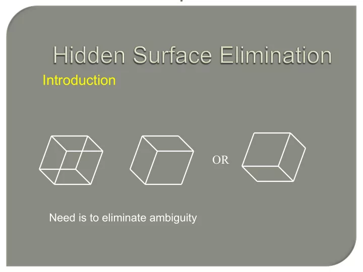
Introduction OR Need is to eliminate ambiguity Introduction Wire frame Hidden Line Elimination Hidden Surface Elimination Introduction Approaches Image Space Through pixel Object Space Through primitive Image Space Approach for (


slide-1
SLIDE 1

Introduction

Need is to eliminate ambiguity

OR

slide-2
SLIDE 2

Introduction

Wire frame Hidden Line Elimination Hidden Surface Elimination

slide-3
SLIDE 3

Introduction

Approaches

  • Image Space

Through pixel

  • Object Space

Through primitive

slide-4
SLIDE 4

Image Space Approach

for (each pixel in the image) { determine the object closest to the viewer that is intercepted by the projector through the pixel; draw the pixel in the appropriate color; }

Computational effort: np n : number of objects p : number of pixels

slide-5
SLIDE 5

Object Space Approach

for (each object in the world) { determine those parts of the object whose view is unobstructed by other parts of it or any other object; draw those parts in the appropriate color; }

Computational effort: n2 n: number of objects

slide-6
SLIDE 6

Floating Horizon Algorithm

Surface Function F(x,y,z)=0

x z z1= constant z2 z3 x y z z1= constant z2 z3 z4 z5

slide-7
SLIDE 7

Floating Horizon Algorithm

With z=constant plane closest to the viewpoint, the curve in each plane is generated (for each x coordinate in image space the appropriate y value is found).

x y z1 z2 z3 z4 z5 Projection on z=0 plane

Algorithm: If at any given value of x the y value

  • f the curve in the current plane is

larger than the y value for any previous curve at that x value, then the curve is visible,

  • therwise it is hidden.
slide-8
SLIDE 8

Floating Horizon Algorithm

x y z1 z2 z3 z4 z5 Projection on z=0 plane

Algorithm: If at any given value of x the y value

  • f the curve in the current plane is

larger than the y value or smaller than the minimum y value for any previous curve at that x value, then the curve is visible,

  • therwise it is hidden.
slide-9
SLIDE 9

Back Face Culling

Preprocessing to eliminate faces which are not visible

P

np

If a surface’s normal is pointing away from the eye (viewer), then this is a back face

backface then V n If

p

< ⋅

V

slide-10
SLIDE 10

Back Face Culling

z x

Conservative algorithm

slide-11
SLIDE 11

Back Face Culling

z x

Conservative algorithm

slide-12
SLIDE 12

Z-Buffer Algorithm

Proposed by Catmull 1974 Simple to implement Z-buffer is like a frame buffer, contains depth

Zb(x, y) C(x, y) (x, y)

(x, y)

slide-13
SLIDE 13

Z-Buffer Algorithm

Initialize all d[i,j]=1.0 (max depth), c[i,j]=background color. for (each polygon) for (each pixel in polygon’s projection) { Find depth-z of polygon at (x,y) corresponding to pixel (i,j); If z < d[i,j] d[i,j] = z; p[i,j] = color; end }

slide-14
SLIDE 14

Z-Buffer Algorithm

1) x ( C A z x C A z z x C A z z C D By x) x A z x x At C C D By Ax z x At D Cz By Ax = − = − = − = − + + + − = + ≠ + + − = = + + + Δ Δ Δ ) Δ ( ( Δ , ) (

1 1 1

Computationally

slide-15
SLIDE 15

Z-Buffer Algorithm

Example

T h e i

T he i m

T h e i m

T he i m ag

T h e i m

T he i m ag

T h e i

T he i m

T h e i

T he i m

T h e i m

T he i m ag

T h e i m

T he i m ag

T h e i

T he i m

T h e i

T he i m

T h e i m

T he i m ag

T h e i m

T he i m ag

T h e i

T he i m

T h e i

T he i m

T h e i m

T he i m ag

T h e i m

T he i m ag

T h e i m T he i m ag T h e i m T he i m ag

Z-buffer Screen

slide-16
SLIDE 16

Z-Buffer Algorithm

Example

[0,1,5] [0,7,5] [6,7,5]

5

T h e i

5

T h e i

T h e i m

5

T he i m ag

5

T h e i m

T h e i m

T h e i

5

T he i m

T h e i

T h e i

T h e i m

T he i m ag

T h e i m

T h e i m

T h e i

T he i m

T h e i

T h e i

T h e i m

T he i m ag

T h e i m

T h e i m

T h e i

T he i m

T h e i

T h e i

T h e i m

T he i m ag

T h e i m

T h e i m

∞ Z-buffer

slide-17
SLIDE 17

Z-Buffer Algorithm

Example

[0,1,2] [0,6,7] [5,1,7]

slide-18
SLIDE 18

Z-Buffer Algorithm

Example

T h e i

5

T he i m

5

T h e i

5

T h e i

5

T h e i m

5

T he i m ag

5

T h e i m

5

T h e i m

5

T h e i

5

T he i m

5

T h e i

5

T h e i

5

T h e i m

5

T he i m ag

5

T h e i m

5

T h e i m

5

T h e i

4

T he i m

5

T h e i

5

T h e i

7

T h e i m

3

T he i m ag

4

T h e i m

5

T h e i m

6

T h e i

2

T he i m

3

T h e i

4

T h e i

5

T h e i m

T he i m ag

T h e i m

T h e i m

T h e i

5

T he i m

5

T h e i

5

T he i m

T h e i m

5

T he i m ag

5

T h e i m

T he i m ag

T h e i

5

T he i m

T h e i

T he i m

T h e i m

T he i m ag

T h e i m

T he i m ag

T h e i

T he i m

T h e i

T he i m

T h e i m

7

T he i m ag

T h e i m

T he i m ag

T h e i

6

T he i m

7

T h e i

T he i m

T h e i m

T he i m ag

T h e i m

T he i m ag

∞ Z-buffer Screen

slide-19
SLIDE 19

Z-Buffer Algorithm

  • Simple method
  • Complexity

Time : nxm buffer k poygons O(nmk) Space : b depth precision O(nmb)

slide-20
SLIDE 20

Painter’s Algorithm

Depth Sort, List Priority Polygons are painted to the screen in the order of their distance from the viewer (More distant objects are painted first)

Screen display

slide-21
SLIDE 21

Painter’s Algorithm

  • Sort polygons in order of increasing depth
  • Draw polygons in sequence, starting from the polygon

(surface) of greatest depth

  • Careful processing of depth
  • Efficiency depends on sorting algorithm
slide-22
SLIDE 22

Painter’s Algorithm

Z=20 Z=15 Z=10

slide-23
SLIDE 23

Painter’s Algorithm

P Q R z P > Q > R P Q z P > Q

Draw first P then Q and then R Draw first P then Q

slide-24
SLIDE 24

Painter’s Algorithm

P Q

Cyclic overlapping May require splitting

slide-25
SLIDE 25

Binary Space Partitioning (BSP)

BSP Tree Space partitioning using planes

slide-26
SLIDE 26

Binary Space Partitioning (BSP)

BSP Tree For hidden surface elimination: sets a display order P B F P B F

slide-27
SLIDE 27

Binary Space Partitioning (BSP)

BSP Tree For hidden surface elimination: sets a display order P B F P B F Eye Display order (back to front): BPF

slide-28
SLIDE 28

Binary Space Partitioning

3 5 5b 5a 2 1 4 3 4 5b front back 1 2 5a

Example

slide-29
SLIDE 29

Binary Space Partitioning

3 5 5b 5a 2 1 4 3 4 5b front back 2 5a 1

Example

slide-30
SLIDE 30

Binary Space Partitioning

3 3 5 5b 5a 2 1 4 front back 2 5a 1 4 5b

Example

slide-31
SLIDE 31

Binary Space Partitioning

3 3 5 5b 5a 2 1 4 front back 2 5a 1 4 5b

Example Display order: 5a 2 1 3 5b 4 V

slide-32
SLIDE 32

Binary Space Partitioning

3 5 2 1 4 5 front back 1 2 3 4

Example

slide-33
SLIDE 33

Binary Space Partitioning

3 5 2 1 4 5 front back 1 2 3 4

Example V Display order: 5 2 1 3 4

slide-34
SLIDE 34

Binary Space Partitioning

Issues How to select the root polygon? Criteria: Number of split (fragmentation)

  • a. Arbitrary
  • b. Heuristic based with 4-5 polygons and consider which gives

the leastnumber of split Static vs Dynamic scene

slide-35
SLIDE 35

Area Subdivision

Quad tree

slide-36
SLIDE 36

Area Subdivision Algorithm

Warnock’s Algorithm

Polygon Area of interest Surrounding Intersecting Contained Disjoint

slide-37
SLIDE 37

Area Subdivision Algorithm

Consider an area of the projected image

If it is easy to decide which polygons are visible in the area, display Else the area is subdivided into smaller areas and the decision is made recursively

Divide and Conquer

slide-38
SLIDE 38

Area Subdivision Algorithm

No Subdivision is required if

  • 1. All the polygons are disjoint: background color in the area.
  • 2. Only one intersecting or only one contained polygon: The area is

filled first by background color, then the polygon part contained in the area.

  • 3. Only one surrounding polygon (no contained and intersecting

polygons): The area is filled with the color of the surrounding polygon.

  • 4. More than one polygon is intersecting, contained in, or

surrounding the area, with surrounding polygon in front: Fill the area with the color of the surrounding polygon.

slide-39
SLIDE 39

Warnock’s Algorithm

Area

slide-40
SLIDE 40

Warnock’s Algorithm

slide-41
SLIDE 41

Warnock’s Algorithm

slide-42
SLIDE 42

Warnock’s Algorithm

slide-43
SLIDE 43

Warnock’s Algorithm

Maximum subdivision: pixel!

slide-44
SLIDE 44

Weiler Atherton Algorithm

Subdivision along polygon boundaries Clipping!

slide-45
SLIDE 45

Weiler Atherton Algorithm

  • Initial z-sort
  • Consider front most polygon, clip all polygons to generate

Fragments inside polygon and outside polygon

  • All inside polygons if behind delete from the list
  • If there is an inside polygon in front (offending), clip the

inside list of polygons against this polygon

  • Process the outside polygon(s)
slide-46
SLIDE 46

Weiler Atherton Algorithm

A BinA BoutA A as clip polygon Inside list: A, BinA Outside list: BoutA Display A Process BoutA

slide-47
SLIDE 47

Weiler Atherton Algorithm

A B x y z x y z A B

slide-48
SLIDE 48

Weiler Atherton Algorithm

A as clip polygon Inside list: A, BinA Outside list: BoutA BinA BoutA BinA as clip polygon Inside list: BinA, AinB Outside list: BoutA, AoutB Display BinA

slide-49
SLIDE 49

Weiler Atherton Algorithm

More polygons with more fragments

slide-50
SLIDE 50

Based on Scan-line coherence across multiple scan-lines or span-coherence ! – scan-conversion algorithm and a little more data structure

Hidden Surface Elimination

Scan Line Algorithm

slide-51
SLIDE 51

Scan Line Algorithm

Spans

slide-52
SLIDE 52

ž Each scan line is subdivided into several "spans" ž Determine which polygon the current span belongs to ž Shade the span using the current polygon’s color ž Exploit "span coherence" : ž For each span, a visibility test may need to be done

Scan Line Algorithm

Overview

slide-53
SLIDE 53

Scan Line Algorithm

slide-54
SLIDE 54

ž A scan line is subdivided into a sequence of spans ž Each span can be "inside" or "outside" polygon areas

  • "outside“: no pixels need to be drawn (background

color)

  • "inside“: can be inside one or multiple polygons

ž If a span is inside one polygon, the pixels in the span will

be drawn with the color of that polygon

ž If a span is inside more than one polygon, then compare

the z values of those polygons at the scan line edge intersection point to determine the color of the pixel

Scan Line Algorithm

Inside/Outside Spans

slide-55
SLIDE 55

ž When a scan line intersects an edge of a polygon

  • for the 1st time, the span becomes "inside" of the

polygon from that intersection point on

  • for a 2nd time, the span becomes "outside“ of the

polygon from that point on

ž A flag "in/out" for each polygon is used to keep track of the

current state

ž Initially, the in/out flag is set to be "outside" (value = 0 for

example). Invert the tag for “inside”.

Hidden Surface Elimination

Scan Line Algorithm

Inside/Outside Spans

slide-56
SLIDE 56

ž Each polygon will have its own in/out flag ž There can be more than one polygon having the in/out

flags to be "in" at a given instance

ž Keep track of polygons the scan line is currently in ž If there are more than one polygon "in", perform z value

comparison to determine the color of the scan line span

Hidden Surface Elimination

Scan Line Algorithm

slide-57
SLIDE 57

Hidden Surface Elimination

Scan Line Algorithm

Data Structure

Edge Table (ET) Polygon Table (PT)

x ymax Δx poly-ID ET PT poly-ID A,B,C,D color in/out flag

slide-58
SLIDE 58

In addition, Use active In-Polygon List (IPL) Active Edge Table (AET)

Hidden Surface Elimination

Scan Line Algorithm

slide-59
SLIDE 59

Example

Hidden Surface Elimination

Scan Line Algorithm S T

a b c 1 2 3 X0 I III II IV XN

BG

slide-60
SLIDE 60

Y AET IPL I x0, ba, bc, xN

BG, BG+S, BG

II x0, ba, bc, 32, 13, xN

BG, BG+S, BG, BG+T, BG

III x0, ba, 32, ca, 13, xN

BG, BG+S, BG+S+T, BG+T, BG

IV x0, ba, ac, 12, 13, xN

BG, BG+S, BG, BG+T, BG

Hidden Surface Elimination

Scan Line Algorithm

Example

slide-61
SLIDE 61

S T

a b c 1 2 3 X0 I III II IV XN

BG

Hidden Surface Elimination

Scan Line Algorithm

Y AET IPL I x0, ba, bc, xN BG, BG+S, BG

Example

slide-62
SLIDE 62

Hidden Surface Elimination

Scan Line Algorithm

Y AET IPL II x0, ba, bc, 32, 13, xN

BG, BG+S, BG, BG+T, BG

Example

S T

a b c 1 2 3 X0 I III II IV XN

BG

slide-63
SLIDE 63

Hidden Surface Elimination

Scan Line Algorithm

Y AET IPL III x0, ba, 32, ca, 13, xN

BG, BG+S, BG+S+T, BG+T, BG

Example

S T

a b c 1 2 3 X0 I III II IV XN

BG

slide-64
SLIDE 64

Hidden Surface Elimination

Scan Line Algorithm

Y AET IPL IV x0, ba, ac, 12, 13, xN

BG, BG+S, BG, BG+T, BG

Example

S T

a b c 1 2 3 X0 I III II IV XN

BG

slide-65
SLIDE 65

Hidden Surface Elimination

Scan Line Algorithm

Non penetrating

slide-66
SLIDE 66

Hidden Surface Elimination

Scan Line Algorithm

I x0, ba , 23, ec, ad, 13, xN BG, BG+S, BG+S+T, BG+S+T+, BG+T, BG Penetrating

S

I

T

a 2

BG

b c 3 d e 1

slide-67
SLIDE 67