Introduction. Historically, there are many episodes/cases of - PDF document

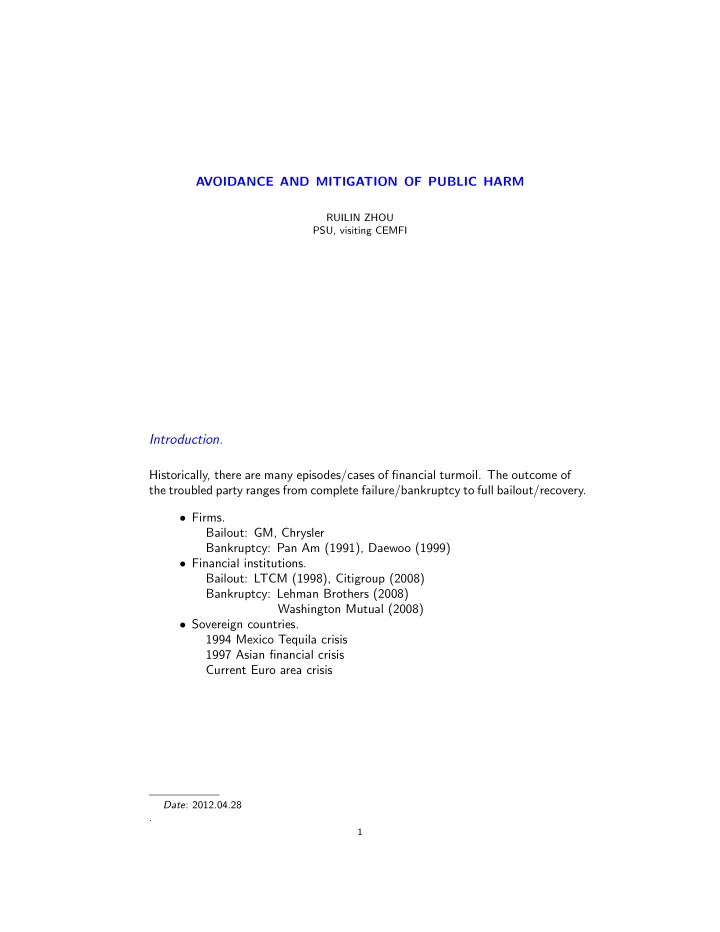
AVOIDANCE AND MITIGATION OF PUBLIC HARM RUILIN ZHOU PSU, visiting CEMFI Introduction. Historically, there are many episodes/cases of financial turmoil. The outcome of the troubled party ranges from complete failure/bankruptcy to full bailout/recovery. • Firms. Bailout: GM, Chrysler Bankruptcy: Pan Am (1991), Daewoo (1999) • Financial institutions. Bailout: LTCM (1998), Citigroup (2008) Bankruptcy: Lehman Brothers (2008) Washington Mutual (2008) • Sovereign countries. 1994 Mexico Tequila crisis 1997 Asian financial crisis Current Euro area crisis Date : 2012.04.28 . 1

2 Two conflicting views about bailout: • Financial turmoil/failures often would generate too much negative ex- ternality, so bailout is beneficial and sometimes necessary ex-post. Too- big-to-fail is consistent with this view. • Bailout creates moral hazard problem: institutions have less incentive to be diligent to reduce crisis incidence since they know that they will be bailed out. A third view: • The observed pattern of bailing out some troubled institutions, but not others, is consistent with the view that the optimal bailout policy is a mixed strategy that deals with both views above. Research program • Construct a schematic, non-cooperative, 2-player model – One agent takes costly, unobservable action to try to avert a crisis. – If the crisis occurs, both agents decide how much to contribute mitigating it. • Characterize Nash equilibrium of the one-shot game: both bailout and no-bailout equilibria always exist. • Consider an infinite repetition of the one-shot stage game – Study in particular equilibrium that minimizes expected, discounted total cost. – Is some equilibrium consistent with the third view?

3 The one-shot game • Two agents. agent 1 — active agent 2 — passive • Two periods. Period 1: • Agent 1 chooses a ∈ A = { 0 , 1 } (avoidance/no avoidance) The cost of avoidance is d . • The state ξ ∈ X = { 0 , 1 } is realized. Pr ( ξ = 1 | a = 0) = 1 Pr ( ξ = 1 | a = 1) = ε Pr ( ξ = 0 | a = 1) = 1 − ε ε ∈ (0 , 1) . Period 2: • If ξ = 1 (crisis state), the two agents play a mitigation game. Agent i contributes m i ∈ M = [0 , 1]  − m i if m 1 + m 2 ≥ 1  u i (1 , m 1 , m 2 ) = − m i − c i otherwise  • If ξ = 0 , no mitigation is necessary. u i (0 , m 1 , m 2 ) = − m i Assumption 1. c i ∈ (0 , 1) for i = 1 , 2 . c 1 + c 2 > 1 .

4 Nash equilibrium of the one-shot game Period 2. Mitigation game. Agent i ’s period-2 strategy m i ( ξ ) , m i : X → M . When ξ = 0 , no need to contribute, m ∗ 1 (0) = m ∗ 2 (0) = 0 . When ξ = 1 , two types of Nash equilibrium. • No-bailout: neither agent contributes anything, m o 1 (1) = m o 2 (1) = 0 u i (1 , m o 1 (1) , m o 2 (1)) = − c i . • Bailout: jointly contribute 1 unit to mitigate m b m b 2 (1) = 1 − m b 1 (1) ∈ [1 − c 2 , c 1 ] , 1 (1) u i (1 , m b 1 (1) , m b 2 (1)) = − m b i (1) Period 1. Agent 1’s avoidance decision a ∈ A . v i ( a, m 1 , m 2 ) —the expected value of agent i in period 1 if • agent 1 takes period-1 action a , • two agents’ strategy in period 2 is ( m 1 ( ξ ) , m 2 ( ξ )) ξ ∈ X . � Pr ( ξ | a ) u 1 ( ξ, m 1 ( ξ ) , m 2 ( ξ )) − ad v 1 ( a, m 1 , m 2 ) = ξ ∈ X � v 2 ( a, m 1 , m 2 ) = Pr ( ξ | a ) u 2 ( ξ, m 1 ( ξ ) , m 2 ( ξ )) ξ ∈ X Agent 1’s optimal period-1 action a depends on which of the period-2 equilib- rium is to be played in case of crisis.

5 If no-bailout equilibrium ( m o 1 (1) , m o 2 (1)) is anticipated,  − c 1 if a = 0  v 1 ( a, m o 1 , m o 2 ) = − d − εc 1 if a = 1   d 1 if c 1 ≥ 1 − ε  a o = the optimal action is 0 otherwise  If the bailout equilibrium ( m b 1 (1) , m b 2 (1)) is anticipated,  − m 1 if a = 0  v 1 ( a, m b 1 , m b 2 ) = − d − εm 1 if a = 1  d  1 if m 1 ≥ 1 − ε  a b = the optimal action is 0 otherwise  Table 1. Equilibrium of the one-shot game parameter range a m 1 (1) ex-ante cost d (1) 1 − ε ≤ 1 − c 2 1 [1 − c 2 , c 1 ] d + ε 1 0 d + ε ( c 1 + c 2 ) d d (2) 1 − c 2 < 1 − ε ≤ c 1 1 [ 1 − ε , c 1 ] d + ε d 0 [1 − c 2 , 1 − ε ] 1 1 0 d + ε ( c 1 + c 2 ) d (3) c 1 < 0 [1 − c 2 , c 1 ] 1 1 − ε 0 0 c 1 + c 2 • By Assumption 1, 0 < 1 − c 2 < c 1 < 1 . • Regardless of the parameter region, both bailout and no-bailout equi- librium always exist. • Any combination of avoidance and mitigation can occur.

6 Ex-ante expected total cost of ( a, m 1 , m 2 ) = ad + (1 − a + aε )[ m 1 + m 2 + ( c 1 + c 2 ) I { m 1 + m 2 < 1 } ] An action profile ( a, m 1 , m 2 ) is said to ex-ante dominate another one if it has a lower expected total cost. • Assumption 1 says that bailout dominates no-bailout ex-post ( c 1 + c 2 > 1 ). In region (1) and (3), bailout also dominates ex-ante. • In region (2), avoidance/bailout achieves the lowest ex-ante expected total cost among all equilibria. The ranking of the other two types of equilibrium is unclear. The repeated game Time is discrete, t = 1 , 2 , . . . . At each date t , the two-period one-shot game is played between the two players with discount factor δ ∈ (0 , 1) . Public information. • At t , h t = ( ξ t , m t 1 , m t 2 ) ∈ H ≡ X × M 2 . • History of public information at the beginning of date t , h t = ( h 1 , . . . , h t − 1 ) ∈ H t − 1 H 0 = ∅ . • When agents decide ( m t 1 , m t 2 ) , the public information is ( h t , ξ t ) ∈ H t − 1 × X .

7 Private information. • Agent 1’s avoidance decision { a t } ∞ t =1 is private and never revealed. A strategy is public if it depends only on public history. Without loss of generality, focus on perfect Bayesian equilibrium where both agents play public strategies. Strategy profile ( α, σ ) = ( α, σ 1 , σ 2 ) = ( α t , σ t 1 , σ t 2 ) ∞ t =1 α t : H t − 1 → ∆( A ) α 1 ∈ ∆( A ) , ∀ t > 1 , for i = 1 , 2 , σ ti : H t − 1 × X → M σ 1 i : X → M, ∀ t > 1 , Let Σ i denote the set of agent i ’s public strategies. Expected present discounted value of payoff stream induced by strategy profile ( α, σ ) , V ( a, σ ) = ( V 1 ( α, σ ) , V 2 ( a, σ )) , ∞ � δ t − 1 � α t ( h t )( a ) v i ( a, σ t ( h t , ξ t ))] V i ( α, σ ) = (1 − δ ) E [ t =1 a ∈ A For any public history h t , let ( α | h t , σ | h t ) denote the strategy profile induced by ( α, σ ) after t periods of history.

8 Definition 1. A public strategy profile ( α ∗ , σ ∗ ) is a perfect public equilibrium (PPE) if ∀ t ≥ 1 , ∀ h t ∈ H t − 1 , ( α ∗ | h t , σ ∗ | h t ) is a Nash equilibrium from t on, that is, for i = 1 , 2 , for any other public strategy ( α, σ 1 ) ∈ Σ 1 , σ 2 ∈ Σ 2 , V 1 ( α ∗ | h t , σ ∗ 1 | h t , σ ∗ 2 | h t ) ≥ V 1 ( α | h t , σ 1 | h t , σ ∗ 2 | h t ) V 2 ( α ∗ | h t , σ ∗ 1 | h t , σ ∗ 2 | h t ) ≥ V 2 ( α ∗ | h t , σ ∗ 1 | h t , σ 2 | h t ) and ∀ ξ t ∈ X , (1 − δ ) u 1 ( ξ t , σ ∗ t 1 , σ ∗ t 2 ) + δV 1 ( α ∗ | h ( t +1) ∗ , σ ∗ 1 | h ( t +1) ∗ , σ ∗ 2 | h ( t +1) ∗ ) ≥ (1 − δ ) u 1 ( ξ t , σ t 1 , σ ∗ t 2 ) + δV 1 ( α | h ( t +1)1 , σ 1 | h ( t +1)1 , σ ∗ 2 | h ( t +1)1 ) (1 − δ ) u 2 ( ξ t , σ ∗ t 1 , σ ∗ t 2 ) + δV 2 ( α ∗ | h ( t +1) ∗ , σ ∗ 1 | h ( t +1) ∗ , σ ∗ 2 | h ( t +1) ∗ ) ≥ (1 − δ ) u 2 ( ξ t , σ ∗ t 1 , σ t 2 ) + δV 1 ( α ∗ | h ( t +1)2 , σ ∗ 1 | h ( t +1)2 , σ 2 | h ( t +1)2 ) where h ( t +1) ∗ = ( h t , ξ t , σ ∗ t 1 , σ ∗ t 2 ) h ( t +1)1 = ( h t , ξ t , σ t 1 , σ ∗ h ( t +1)2 = ( h t , ξ t , σ ∗ t 2 ) , t 1 , σ t 2 ) A PPE always exists: repetition of any static Nash equilibrium of the two-period stage game is a PPE. Let V denote the set of PPE payoff vectors, V = { V ( α, σ ) | ( α, σ ) is a PPE } V � = ∅ . Following APS (1990), find V through a self-generation procedure. Define expected payoff of action profile ( φ, m 1 , m 2 ) if continuation value is w : X × M 2 → ℜ 2 , for i = 1 , 2 , � � g i ( φ, m 1 , m 2 , w ) ≡ φ ( a ) (1 − δ ) v i ( a, m 1 , m 2 ) a ∈ A � � + δ Pr ( ξ | a ) w i ( ξ, m 1 ( ξ ) , m 2 ( ξ )) ξ ∈ X

9 For any W ⊂ ℜ 2 , an action profile ( φ, m 1 , m 2 ) together with Definition 2. payoff function w : X × M 2 → ℜ 2 is admissible with respect to W if (1) ∀ ξ ∈ X , w ( ξ, m 1 ( ξ ) , m 2 ( ξ )) ∈ W . 1 ( ξ ) ∈ M } ξ ∈ X g 1 ( φ ′ , m ′ (2) ( φ, m 1 ) = arg max φ ′ ∈ ∆( A ) , { m ′ 1 , m 2 , w ) (3) For any ξ ∈ X , for any m ′ 1 and m ′ 2 , (1 − δ ) u 1 ( ξ, m 1 ( ξ ) , m 2 ( ξ )) + δw 1 ( ξ, m 1 ( ξ ) , m 2 ( ξ )) ≥ (1 − δ ) u 1 ( ξ, m ′ 1 ( ξ ) , m 2 ( ξ )) + δw 1 ( ξ, m ′ 1 ( ξ ) , m 2 ( ξ )) (1 − δ ) u 2 ( ξ, m 1 ( ξ ) , m 2 ( ξ )) + δw 2 ( ξ, m 1 ( ξ ) , m 2 ( ξ )) ≥ (1 − δ ) u 2 ( ξ, m 1 ( ξ ) , m ′ 2 ( ξ )) + δw 2 ( ξ, m 1 ( ξ ) , m ′ 2 ( ξ )) For any W ⊂ ℜ 2 , define � B ( W ) = r | ∃ ( φ, m 1 , m 2 , w ) admissible w . r . t . W � such that r = g ( φ, m 1 , m 2 , w ) Then B ( V ) = V . The set of PPE payoff vectors V can be obtained numerically by starting from some initial set W 0 ⊂ ℜ 2 , B t ( W 0 ) → V as t → ∞