[PPT] - Internal Model Principle 1. v G c ( z ) = S c G ( z ) = B r e u PowerPoint Presentation

SLIDE 1

1. Internal Model Principle

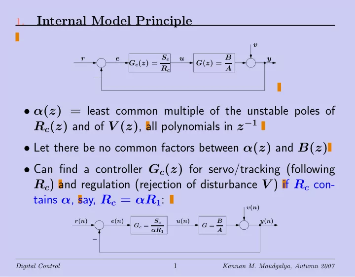
r − G(z) = B A Gc(z) = Sc Rc u e y v

α(z) = least common multiple of the unstable poles of

Rc(z) and of V (z), all polynomials in z−1

Let there be no common factors between α(z) and B(z)
Can find a controller Gc(z) for servo/tracking (following

Rc) and regulation (rejection of disturbance V ) if Rc con- tains α, say, Rc = αR1:

e(n) − y(n) G = B A r(n) Gc = Sc αR1 u(n) v(n)

Digital Control

1 Kannan M. Moudgalya, Autumn 2007

SLIDE 2

2. Internal Model Principle - Regulation

e(n) − y(n) G = B A r(n) Gc = Sc αR1 u(n) v(n)

Y (z) = Sc R1 1 α B A 1 + Sc R1 1 α B A R + 1 1 + Sc R1 1 α B A V = ScB R1Aα + ScBR + R1Aα R1Aα + ScB bV αaV

Unstable pole present in α gets cancelled
Regulation problem verified

Digital Control

2 Kannan M. Moudgalya, Autumn 2007

SLIDE 3

3. Internal Model Principle - Servo

e(n) − y(n) G = B A r(n) Gc = Sc αR1 u(n) v(n)

Y (z) = ScB R1Aα + ScBR + R1Aα R1Aα + ScBV Servo problem: assume V = 0: E(z) = R(z) − Y (z) =

1 −

ScB R1Aα + ScB

R =

R1Aα R1Aα + ScB bR αaR

Unstable poles of Rc are cancelled by zeros of α.
Can choose Rc and Sc such that R1Aα + ScB has roots

within the unit circle (pole placement)

IM Principle: unstable poles of V , Rc appear in loop thro’

α

Digital Control

3 Kannan M. Moudgalya, Autumn 2007

SLIDE 4

4. Internal Stability

u(n) e(n) − y(n) + r(n) gc(n) g(n)

Notion in UG classes: output has to be stable
Output being stable is not sufficient
Every signal in the loop should be bounded
If any signal is unbounded, will result in saturation / overflow

/ explosion

When every signal is bounded, called internal stability
If output is stable and if there is no unstable pole-zero can-

cellation, internal stability

Digital Control

4 Kannan M. Moudgalya, Autumn 2007

SLIDE 5

5.

Unstb. Pole-Zero Cancel. = No Int. Stability

+ − + r1 Gc = n2 d2 r2 G = n1 d1 e1 e2 y +

E1 E2

=

    1 1 + GGc − G 1 + GGc Gc 1 + GcG 1 1 + GcG     R1 R2

=

    d1d2 n1n2 + d1d2 − n1d2 n1n2 + d1d2 n2d1 n1n2 + d1d2 d1d2 n1n2 + d1d2     R1 R2

Suppose d1, n2 have a common factor:

d1 = (z + a)d′

1

n2 = (z + a)n′

2 Digital Control

5 Kannan M. Moudgalya, Autumn 2007

SLIDE 6

6. Unstable Pole-Zero Cancellation = No Internal Stability Assume the cancellation of z + a, G(z) = n1(z) (z + a)d′

1(z),

Gc(z) = (z + a)n′

2(z)

d2(z) with |a| > 1. Assume stability of TE = 1 1 + GGc = d′

1d2

d′

1d2 + n1n′ 2

T.F. between R2 and Y can be shown to be unstable. Let R1 = 0. Y R2 = G 1 + GGc = n1d2 (d′

1d2 + n1n′ 2)(z + a)

It is unstable and a bounded signal injected at R2 will produce an unbounded signal at Y

Digital Control

6 Kannan M. Moudgalya, Autumn 2007

SLIDE 7

7. Forbid Unstable Pole-Zero Cancellation: Loop Variable

Internal stability = all variables in loop are bounded for bounded

external inputs at all locations

Can be checked by the following closed loop diagram

+ − + r1 Gc = n2 d2 r2 G = n1 d1 e1 e2 y +

Can show that Output is stable + no pole-zero cancellation

= internal stability

Digital Control

7 Kannan M. Moudgalya, Autumn 2007

SLIDE 8

8. Forbid Unstable Pole-Zero Cancellation ⇒ Get Causality Not possible to realize this controller: Gc = 1 + z−1 z−1 All sampled systems have at least one delay: G(z−1) = z−kB(z−1) A(z−1) = z−kb0 + b1z−1 + b2z−2 + · · · 1 + a1z−1 + a2z−2 + · · ·

Controller not realizable ⇒ there is a common factor z−1

between plant and controller

z−1 = 0 ⇒ z = ∞, an unstable pole
If unstable pole-zero cancellation is forbidden while designing

controllers, z−1 cannot appear in the denominator of the controller - i.e., controller is realizable

Digital Control

8 Kannan M. Moudgalya, Autumn 2007

SLIDE 9

9. Delay Specification for Realizability Closed loop delay has to be ≥ open loop delay: G(z) = z−kB(z) A(z) = z−kb0 + b1z−1 + · · · 1 + a1z−1 + · · · b0 = 0. Suppose that we use a feedback controller of the form Gc(z) = z−d Sc(z) Rc(z) = z−ds0 + s1z−1 + · · · 1 + r1z−1 + · · · with s0 = 0 and d ≥ 0. Closed loop transfer function: T = GGc 1 + GGc = z−k−d b0s0 + (b0s1 + b1s0)z−1 + · · · 1 + (s1 + r1)z−1 + · · · + z−k−d(b0s0 + · · · )

Digital Control

9 Kannan M. Moudgalya, Autumn 2007

SLIDE 10

10. Delay Specification for Realizability T = z−k−d b0s0 + (b0s1 + b1s0)z−1 + · · · 1 + (s1 + r1)z−1 + · · · + z−k−d(b0s0 + · · · )

Closed loop delay = k + d ≥ k = open loop delay.
Can make it less only by d < 0, but controller is unrealizable.

Digital Control

10 Kannan M. Moudgalya, Autumn 2007

SLIDE 11

11. Example: What if Wrong Delay is Specified? Design a controller for the plant G = z−2 1 1 − 0.5z−1 so that the overall system has smaller delay: T = z−1 1 1 − az−1 Recall the standard closed loop transfer function: T = GGc/(1+ GGc). Solving for Gc, and substituting for T , G Gc = 1 G T 1 − T = 1 z−1 1 − 0.5z−1 1 − (a + 1)z−1 This controller is unrealizable, no matter what a is.

Digital Control

11 Kannan M. Moudgalya, Autumn 2007

SLIDE 12

12. Specifications - Step Response Give unit step input in r. Output y should have

1. small rise time
2. small overshoot
3. small settling time
4. small steady state error

n e(n) n y(n)

Error e(n) of the following form sat- isfies the requirements: e(n) = ρn cos ωn, 0 < ρ < 1

× × ω ρ Im(z) Re(z)

Digital Control

12 Kannan M. Moudgalya, Autumn 2007

SLIDE 13

13. Specifications - Step Response

n e(n) n y(n)

× × ω ρ Im(z) Re(z)

e(n) = ρn cos ωn 0 < ρ < 1

1. initial error is one
2. decaying oscillations about zero
3. steady state error is zero

Procedure: User will specify the following:

1. a maximum allowable fall time < Nr
2. a maximum allowable undershoot < ε
3. a minimum required decay ratio < δ
We will develop a method to determine ρ and

ω satisfying the above requirements

Calculate trans. fn. between e(n) - r(n
Back calculate the controller Gc(z)

Digital Control

13 Kannan M. Moudgalya, Autumn 2007

SLIDE 14

14. Small Fall Time in Error e(n) = ρn cos ωn, 0 < ρ < 1 Error becomes zero, i.e., e(n) = 0. for the first time when ωn = π 2 ⇒ n = π 2ω As want n < Nr, some given value, we get π 2ω < Nr ⇒ ω > π 2Nr

n e(n) n y(n)

Desired region:

Im(z) Re(z)

Digital Control

14 Kannan M. Moudgalya, Autumn 2007

SLIDE 15

15. Small Undershoot e(n) = ρn cos ωn When does it reach first min.? de/dn = 0

Not applicable, because n is an integer
Look for a simpler expression
Reaches min. approx. when ωn = π

e(n)|ωn=π = ρn cos ωn|ωn=π = −ρn|ωn=π = −ρπ/ω User specified maximum deviation = ε: ρπ/ω < ε, ρ < εω/π

n e(n) n y(n)

Desired region:

Im(z) Re(z)

Digital Control

15 Kannan M. Moudgalya, Autumn 2007

SLIDE 16

16. Small Decay Ratio e(n) = ρn cos ωn Ratio of two successive peak/trough to be small

First undershoot in e(n) occurs at ωn ≃ π
First overshoot occurs at ωn ≃ 2π

Want this ratio to be less than user specified δ:

e(n)|ωn=2π

e(n)|ωn=π

< δ ⇒ ρn|ωn=2π

ρn|ωn=π < δ δ = 0.5 ≃ 1/4 decay. δ = 0.25 ≃ 1/8 decay. ρ2π/ω ρπ/ω < δ ⇒ ρπ/ω < δ ⇒ ρ < δω/π

Small undershoot: ρ < εω/π. Usually ε < δ
Small undershoot satisfies fast decay

n e(n) n y(n)

Desired region:

Im(z) Re(z)

Digital Control

16 Kannan M. Moudgalya, Autumn 2007

SLIDE 17

17. Overall Requirements

Im(z) Re(z) Im(z) Re(z) Re(z) Im(z)

Desired region by the current approach

Im(z) Re(z)

Obtained by discretization of continuous domain result (Astrom and Wittenmark)

Digital Control

17 Kannan M. Moudgalya, Autumn 2007

SLIDE 18

18. Desired Transfer Function Desired error to a step input is e: e(n) = rn cos ωn Taking Z-transform, E(z) = z(z − r cos ω) z2 − 2zr cos ω + r2 For step input R(z). Transfer function between R(z)-E(z): TE(z) = E(z) R(z) = z(z − r cos ω) z2 − 2zr cos ω + r2 z − 1 z = (z − 1)(z − r cos ω) z2 − 2zr cos ω + r2 One approach: equate this to 1/(1 + GGc) and calculate Gc

Digital Control

18 Kannan M. Moudgalya, Autumn 2007

SLIDE 19

19. Desired Transfer Function Transfer function between setpoint R(z) and actual output Y (z): TY (z) = 1 − TE(z) = 1 − z2 − zr cos ω − z + r cos ω z2 − 2zr cos ω + r2 = z(1 − r cos ω) + (r2 − r cos ω) z2 − 2zr cos ω + r2