Initializing Vectors colon operator x = 1:2:10 Vectors and - PDF document

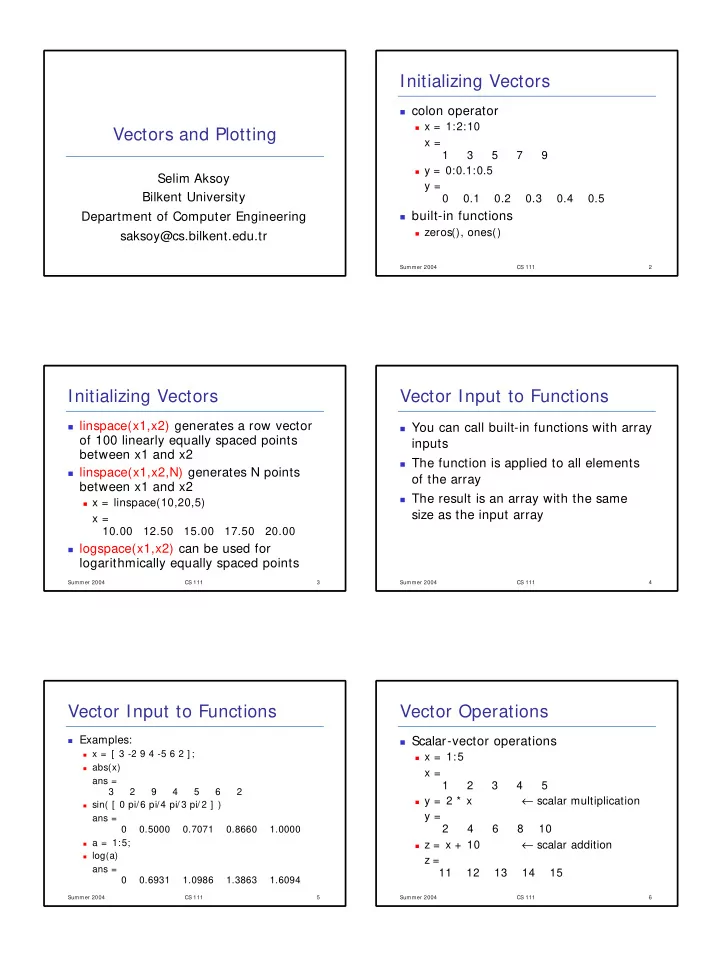
Initializing Vectors � colon operator � x = 1:2:10 Vectors and Plotting x = 1 3 5 7 9 � y = 0:0.1:0.5 Selim Aksoy y = Bilkent University 0 0.1 0.2 0.3 0.4 0.5 Department of Computer Engineering � built-in functions � zeros(), ones() saksoy@cs.bilkent.edu.tr Summer 2004 CS 111 2 Initializing Vectors Vector Input to Functions � linspace(x1,x2) generates a row vector � You can call built-in functions with array of 100 linearly equally spaced points inputs between x1 and x2 � The function is applied to all elements � linspace(x1,x2,N) generates N points of the array between x1 and x2 � The result is an array with the same � x = linspace(10,20,5) size as the input array x = 10.00 12.50 15.00 17.50 20.00 � logspace(x1,x2) can be used for logarithmically equally spaced points Summer 2004 CS 111 3 Summer 2004 CS 111 4 Vector Input to Functions Vector Operations � Examples: � Scalar-vector operations � x = [ 3 -2 9 4 -5 6 2 ] ; � x = 1:5 � abs(x) x = ans = 1 2 3 4 5 3 2 9 4 5 6 2 ← scalar multiplication � y = 2 * x � sin( [ 0 pi/6 pi/4 pi/ 3 pi/2 ] ) y = ans = 2 4 6 8 10 0 0.5000 0.7071 0.8660 1.0000 ← scalar addition � a = 1:5; � z = x + 10 � log(a) z = ans = 11 12 13 14 15 0 0.6931 1.0986 1.3863 1.6094 Summer 2004 CS 111 5 Summer 2004 CS 111 6

Vector Operations Vector Operations � Vector-vector operations � Vector-vector operations (element-by-element operations) (element-by-element operations) � x = [ 1 2 3 4 5 ] ; y = [ 2 -1 4 3 -2 ] ; � z = x .^ y � z = x + y z = � z = 3 1 7 7 3 1.00 0.50 81.00 64.00 0.04 � z = x .* y � Use .* , ./, .^ for element-by-element z = operations 2 -2 12 12 -10 � z = x ./ y � Vector dimensions must be the same z = 0.5000 -2.0000 0.7500 1.3333 -2.5000 Summer 2004 CS 111 7 Summer 2004 CS 111 8 Loops vs. Vectorization Loops vs. Vectorization %Compares execution times of loops and vectors � Problem: Find the maximum value in a % %by Selim Aksoy, 7/3/2004 vector %Create a vector of random values x = rand (1,10000); � Soln. 1: Write a loop %Find the maximum value using a loop tic; %reset the time counter m = 0; � Soln. 2: Use the built -in function “max” for ii = 1:length(x), if ( x(ii) > m ), m = x(ii); � Use built-in MATLAB functions as much end end t1 = toc; %elapsed time since last call to tic as possible instead of reimplementing %Find the maximum using the built-in function tic; %reset the time counter them m = max (x); t2 = toc; %elapsed time since last call to tic %Display timing results fprintf( 'Timing for loop is %f\n', t1 ); fprintf( 'Timing for built-in function is %f\n', t2 ); Summer 2004 CS 111 9 Summer 2004 CS 111 10 Loops vs. Vectorization Loops vs. Vectorization %Compares execution times of loops and vectors � Problem: Compute 3x 2 + 4x+ 5 for a % %by Selim Aksoy, 7/3/2004 %Use a loop given set of values tic; %reset the time counter clear y; for x = 1:10000, � Soln. 1: Write a loop y(x) = 3 * x ^ 2 + 4 * x + 5; end t1 = toc; %elapsed time since last call to tic � Soln. 2: Use 3* x.^ 2 + 4* x + 5 %Use a loop again but also initialize the result vector tic; %reset the time counter clear y; y = zeros (1,10000); � Allocate all arrays used in a loop before for x = 1:10000, y(x) = 3 * x ^ 2 + 4 * x + 5; end executing the loop t2 = toc; %elapsed time since last call to tic %Use vector operations tic; %reset the time counter � If it is possible to implement a clear y; x = 1:10000; y = 3 * x .^ 2 + 4 * x + 5; calculation either with a loop or using t3 = toc; %elapsed time since last call to tic %Display timing results fprintf ( 'Timing for uninizialed vector is % f\n', t1 ) ; vectors, always use vectors fprintf ( 'Timing for inizialed vector is % f\n', t2 ); fprintf ( 'Timing for vectorization is %f\n', t3 ) ; Summer 2004 CS 111 11 Summer 2004 CS 111 12

Plotting Plotting: Multiple Graphs x = linspace(0, 4* pi); x = linspace(0, 4* pi); y = sin(x); y1 = sin(x); plot(x,y); y2 = sin(x) .^ 2; title( 'sin(x) for [0,4\pi]' ); y3 = y1 + y2; xlabel( 'x' ); plot(x,y1,'b-'); ylabel( 'y' ); hold on; grid on; plot(x,y2,'r--'); axis( [ 0 4* pi -1 1 ] ); plot(x,y3,'g:'); hold off; Summer 2004 CS 111 13 Summer 2004 CS 111 14 Plotting: Multiple Graphs Plotting: Subplots x = linspace(0, 4* pi); x = -2:0.1:4; y1 = sin(x); y = 3.5 .^ (-0.5* x) .* ... cos(6* x); y2 = sin(x) .^ 2; figure(1); y3 = y1 + y2; subplot(2,1,1); plot(x,y1,x,y2,x,y3); plot(x,y,'r-o'); legend( 'sin(x)', ... 'sin(x)^ 2', ... subplot(2,1,2); 'sin(x) + sin(x)^ 2' ); plot(x,y,'k--* '); print -f1 -dtiff myplot.tif Summer 2004 CS 111 15 Summer 2004 CS 111 16 Plotting: Logarithmic Plots Plotting Summary r = 16000; c = 1.0e-6; � plot(x,y) f = 1:2:1000; linear plot of vector y vs. vector x res = 1 ./ ( 1 + j* 2* pi* f* r* c ); amp = abs(res); � title('text'), xlabel('text'), ylabel('text') phase = angle(res); subplot (2,1,1); labels the figure, x-axis and y-axis loglog(f,amp); title( 'Amplitude response' ); � grid on/off xlabel( 'Frequency (Hz)' ); adds/removes grid lines ylabel( 'Output/Input ratio' ); grid on; � legend( 'string1', 'string2', 'string3', ... ) subplot (2,1,2); semilogx(f,phase); adds a legend using the specified strings title( 'Phase response' ); xlabel( 'Frequency (Hz)' ); � hold on/off ylabel( 'Output -Input phase (rad)' ); allows/disallows adding subsequent graphs to grid on; the current graph Summer 2004 CS 111 17 Summer 2004 CS 111 18

Plotting Summary Plotting Summary � axis( [ xmin xmax ymin ymax ] ) line color line marker line style sets axes’ limits b blue . point - solid g green o circle : dotted � v = axis r red x x-mark -. dashdot returns a row vector containing the c cyan + plus -- dashed m magenta * star scaling for the current plot y yellow s square � axis equal k black d diamond v triangle (down) sets the same scale for both axes ^ triangle (up) � axis square < triangle (left) > triangle (right) makes the current axis square in size p pentagram h hexagram Summer 2004 CS 111 19 Summer 2004 CS 111 20 Plotting Summary Plotting Summary � semilogy(x,y), semilogx(x,y), loglog(x,y) � print –f< handle> -d< device> < filename> logarithmic plots of vector y vs. vector x saves the figure with the given handle in the format specified by the device � figure(k) makes k the current figure � -deps Encapsulated PostScript � -depsc Encapsulated Color PostScript � subplot(m,n,p) � -deps2 Encapsulated Level 2 PostScript breaks the figure window into an m-by-n � -depsc2 Encapsulated Level 2 Color PostScript matrix of small axes and selects the p th � -djpeg<nn> JPEG image with quality level of nn axes for the current plot � -dtiff TIFF image � clf � -dpng Portable Network Graphics image clears current figure Summer 2004 CS 111 21 Summer 2004 CS 111 22 Plotting Examples Plotting Examples � Vertical bar plot � Line plot y = 1988:1994; x = -2:0.01:4; s = [ 8 12 20 22 18 24 27 ]; y = 3.5.^ (-0.5* x).* cos(6* x); bar(y,s,'r'); plot(x,y); line([0 0],[-3 3],'color','r'); � Pie plot � Horizontal bar plot grades = [ 11 18 26 9 5 ]; y = 1988:1994; pie(grades); s = [ 8 12 20 22 18 24 27 ]; barh(y,s,'g'); Summer 2004 CS 111 23 Summer 2004 CS 111 24

Plotting Examples Plotting Examples � Stairs plot � Histogram y = 1988:1994; x = randn(1,100); s = [ 8 12 20 22 18 24 27 ]; hist(x,10); stairs(y,s); hist(x,20); � Stem plot y = 1988:1994; s = [ 8 12 20 22 18 24 27 ]; stem(y,s); Summer 2004 CS 111 25 Summer 2004 CS 111 26 Plotting Examples Plotting Examples � Polar plot � Error bar plot t = linspace(0,2* pi,200); x = 1:10; r = 3 * cos(0.5* t).^ 2 + t; y = sin(x); polar(t,r); e = std(y) * ones(size(x)); errorbar(x,y,e); � Compass plot u = [ 3 4 -2 -3 0.5 ]; v = [ 3 1 3 -2 -3 ] ; compass(u,v); Summer 2004 CS 111 27 Summer 2004 CS 111 28