Information Theory Lecture 4 Discrete channels, codes and capacity: - - PDF document

Information Theory

Lecture 4

• Discrete channels, codes and capacity: CT7
• Channels: CT7.1–2
• Capacity and the coding theorem: CT7.3–7 and CT7.9
• Combining source and channel coding: CT7.13

Mikael Skoglund, Information Theory 1/19

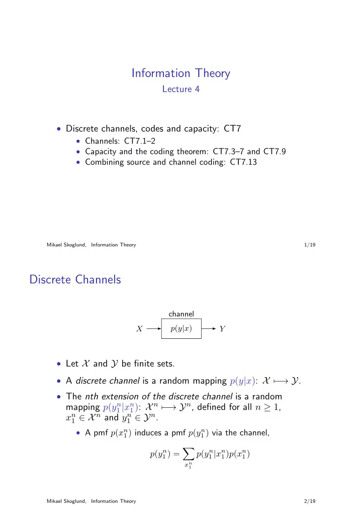
Discrete Channels

X p(y|x) channel Y

• Let X and Y be finite sets.
• A discrete channel is a random mapping p(y|x): X −

→ Y.

• The nth extension of the discrete channel is a random

mapping p(yn

1 |xn 1): X n −

→ Yn, defined for all n ≥ 1, xn

1 ∈ X n and yn 1 ∈ Yn.

• A pmf p(xn

1) induces a pmf p(yn 1 ) via the channel,

p(yn

1 ) =

• xn

1

p(yn

1 |xn 1)p(xn 1)

Mikael Skoglund, Information Theory 2/19

• The channel is stationary if for any n

p(yn

1 |xn 1) = p(yn+k 1+k |xn+k 1+k),

k = 1, 2, . . .

• A stationary channel is memoryless if

p(ym|xm

1 ym−1 1

) = p(ym|xm), m = 2, 3, . . . That is, the channel output at time m does not depend on past inputs or outputs.

• Furthermore, if the channel is used without feedback

p(yn

1 |xn 1) = n

• m=1

p(ym|xm), n = 2, 3, . . . That is, each time the channel is used its effect on the output is independent of previous and future uses.

Mikael Skoglund, Information Theory 3/19

• A discrete memoryless channel (DMC) is completely described

by the triple (X, p(y|x), Y).

• The binary symmetric channel (BSC) with crossover

probability ε,

• a DMC with X = Y = {0, 1} and p(1|0) = p(0|1) = ε

X 1 Y 1 1 − ε ε ε 1 − ε

• The binary erasure channel (BEC) with erasure probability ε,
• a DMC with X = {0, 1}, Y = {0, 1, e} and p(e|0) = p(e|1) = ε

X 1 Y e 1 1 − ε ε ε 1 − ε

Mikael Skoglund, Information Theory 4/19

A Block Channel Code

ω encoder α(·) xn

1 (ω)

channel p(y|x) Y n

1

decoder β(·) ˆ ω

• An (M, n) block channel code for a DMC (X, p(y|x), Y) is

defined by:

1 An index set IM {1, . . . , M}. 2 An encoder mapping α : IM −

→ X n. The set Cn

• xn

1 : xn 1 = α(i), ∀ i ∈ IM

• f codewords is called the codebook.

3 A decoder mapping β : Yn −

→ IM.

• The rate of the code is

R log M n [bits per channel use]

Mikael Skoglund, Information Theory 5/19

Why?

• M different codewords {xn

1(1), . . . , xn 1(M)} can convey log M

bits of information per codeword, or R bits per channel use.

• Consider M = 2k, |X| = 2, and assume that k < n. Then k

“information bits” are mapped into n > k “coded bits.” Introduces redundancy; can be employed by the decoder to correct channel errors.

Mikael Skoglund, Information Theory 6/19

Error Probabilities

• Information symbol ω ∈ IM, with p(i) = Pr(ω = i). Then,

for a given DMC and a given code ω − → Xn

1 = α(ω) −

→ Y n

1

− → ˆ ω = β(Y n

1 )

• Define:

1 The conditional error probability: λi = Pr(ˆ

ω = i|ω = i)

2 The maximal error probability: λ(n) = max {λ1, . . . , λM} 3 The average error probability:

P (n)

e

= Pr(ˆ ω = ω) =

M

• i=1

λi p(i)

Mikael Skoglund, Information Theory 7/19

Jointly Typical Sequences

The set A(n)

ε

• f jointly typical sequences with respect to a pmf

p(x, y) is the set {(xn

1, yn 1 )} of sequences for which

• − 1

n log p(xn

1) − H(X)

• < ε
• − 1

n log p(yn

1 ) − H(Y )

• < ε
• − 1

n log p(xn

1, yn 1 ) − H(X, Y )

• < ε

where p(xn

1, yn 1 ) = n

• m=1

p(xm, ym) p(xn

1) =

• yn

1

p(xn

1, yn 1 ),

p(yn

1 ) =

• xn

1

p(xn

1, yn 1 )

and where the entropies are computed based on p(x, y).

Mikael Skoglund, Information Theory 8/19

The joint AEP Let (Xn

1 , Y n 1 ) drawn according to p(xn 1, yn 1 ) = n m=1 p(xm, ym)

• Pr
• (Xn

1 , Y n 1 ) ∈ A(n) ε

• > 1 − ε for sufficiently large n.
• |A(n)

ε | ≤ 2n(H(X,Y )+ε).

• |A(n)

ε | ≥ (1 − ε)2n(H(X,Y )−ε) for sufficiently large n.

• If ˜

Xn

1 and ˜

Y n

1 are drawn independently according to

p(xn

1) = yn

1 p(xn

1, yn 1 ) and p(yn 1 ) = xn

1 p(xn

1, yn 1 ), then

Pr

• ( ˜

Xn

1 , ˜

Y n

1 ) ∈ A(n) ε

• ≤ 2−n(I(X;Y )−3ε)

and for sufficiently large n Pr

• ( ˜

Xn

1 , ˜

Y n

1 ) ∈ A(n) ε

• ≥ (1 − ε)2−n(I(X;Y )+3ε)

with I(X; Y ) computed for the pmf p(x, y).

Mikael Skoglund, Information Theory 9/19

Channel Capacity

• For a fixed n, a code can convey more information for large

M = ⇒ we would like to maximize the rate R = 1

n log M

without sacrificing performance

• Which is the largest R that allows for a (very) low P (n)

e

??

• For a given channel we say that the rate R is achievable if

there exists a sequence of (M, n) codes, with M = ⌈2nR⌉, such that the maximal probability of error λ(n) → 0 as n → ∞. The capacity C of a channel is the supremum of all rates that are achievable over the channel.

Mikael Skoglund, Information Theory 10/19

Random Code Design

• Choose a joint pmf p(xn

1) on X n.

• Random code design: Draw M codewords xn

1(i), i = 1, . . . ,

M, i.i.d. according to p(xn

1) and let these define a codebook

Cn =

• xn

1(1), . . . , xn 1(M)

• .
• Note: The interpretation here is that the codebook is

“designed” in a random fashion. When the resulting code then is used, the codebook must, of course, be fixed and known. . .

Mikael Skoglund, Information Theory 11/19

A Lower Bound for C of a DMC

• A DMC (X, p(y|x), Y).
• Fix a pmf p(x) for x ∈ X.

Generate Cn = {xn

1(1), . . . , xn 1(M)} using p(xn 1) = p(xm).

• A data symbol ω is generated according to a uniform

distribution on IM, and xn

1(ω) is transmitted.

• The channel produces a corresponding output sequence Y n

1 .

• Let A(n)

ε

be the typical set w.r.t. p(x, y) = p(y|x)p(x). At the receiver, the decoder then uses the following decision

• rule. Index ˆ

ω was sent if:

xn

1(ˆ

ω), Y n

1

• ∈ A(n)

ε

for some small ε;

• no other ω corresponds to a jointly typical
• xn

1(ω), Y n 1

• .

Mikael Skoglund, Information Theory 12/19

Now study πn = Pr(ˆ ω = ω) where “Pr” is over the random codebook selection, the data variable ω and the channel.

• Symmetry =

⇒ πn = Pr(ˆ ω = 1|ω = 1)

• Let

Ei = {(xn

1(i), Y n 1 ) ∈ A(n) ε }

then for a sufficiently large n, πn = P(Ec

1 ∪ E2 ∪ · · · ∪ EM) ≤ P(Ec 1) + M

• i=2

P(Ei) ≤ ε + (M − 1)2−n(I(X;Y )−3ε) ≤ ε + 2−n(I(X;Y )−R−3ε) because of the union bound and the joint AEP.

Mikael Skoglund, Information Theory 13/19

• Note that

I(X; Y ) =

• x,y

p(y|x)p(x) log p(y|x) p(y) with p(y) =

x p(y|x)p(x), where p(x) generated the

random codebook and p(y|x) is given by the channel.

• Let Ctot be the set of all possible codebooks that can be

generated by p(xn

1) = p(xm), then at least one Cn ∈ Ctot

must give P (n)

e

≤ πn ≤ ε + 2−n(I(X;Y )−R−3ε) = ⇒ as long as R < I(X; Y ) − 3ε there exists at least one Cn ∈ Ctot, say C∗

n, that can give P (n) e

→ 0 as n → ∞.

Mikael Skoglund, Information Theory 14/19

• Order the codewords in C∗

n according to the corresponding

λi’s and throw away the worst half = ⇒

• new rate R′ = R − n−1
• for the remaining codewords

λ(n) 2 ≤ ε + 2−n(I(X;Y )−R−3ε)

= ⇒ for any p(x), all rates R < I(X; Y ) − 3ε achievable = ⇒ all rates R < maxp(x) I(X; Y ) − 3ε achievable = ⇒ C ≥ max

p(x) I(X; Y )

Mikael Skoglund, Information Theory 15/19

An Upper Bound for C of a DMC

• Let Cn = {xn

1(1), . . . , xn 1(M)} be any sequence of codes that

can achieve λ(n) → 0 at a fixed rate R = 1

n log M.

• Note that λ(n) → 0 =

⇒ P (n)

e

→ 0 for any p(ω). We can assume Cn encodes equally probable ω ∈ IM.

• Fano’s inequality =

⇒ R ≤ 1 n+P (n)

e

R+ 1 nI(xn

1(ω); Y n 1 ) ≤ 1

n+P (n)

e

R+max

p(x) I(X; Y )

That is, for any fixed achievable R λ(n) → 0 = ⇒ R ≤ max

p(x) I(X; Y ) =

⇒ C ≤ max

p(x) I(X; Y )

Mikael Skoglund, Information Theory 16/19

The Channel Coding Theorem for DMC’s

Theorem (the channel coding theorem)

For a given DMC (X, p(y|x), Y), let p(x) be a pmf on X and let C = max

p(x) I(X; Y )

= max

p(x)

  

• x∈X
• y∈Y

p(y|x)p(x) log p(y|x)

• x∈X p(y|x)p(x)

   Then C is the capacity of the channel. That is, all rates R < C and no rates R > C are achievable.

Mikael Skoglund, Information Theory 17/19

The Joint Source–Channel Coding Theorem

• A (stationary and ergodic) discrete source S with entropy rate

H(S) [bits/source symbol].

• A length-L block of source symbols can be coded into k bits,

and then reconstructed without errors as long as k/L > H(S) and as L → ∞.

• A DMC (X, p(y|x), Y) with capacity C [bits/channel use].
• If k/n < C a channel code exists that can convey k bits of

information per n channel uses without errors as n → ∞.

• L source symbols → k information bits → n channel symbols;

will convey the source symbols without errors as long as H(S) < k L < n L · C

Mikael Skoglund, Information Theory 18/19

• Hence, as long as H(S) < C [bits/source symbol] the source

can be transmitted without errors, as both L → ∞ and n → ∞ (assuming n/L = 1).

• If H(S) > C there is no way of constructing a system with an

error probability that is not bounded away from zero. (Fano’s inequality, etc.)

• No system exists that can communicate a source without

errors for H(S) > C. One way of achieving error-free performance, for H(S) < C, is to use separate source and channel coding.

Mikael Skoglund, Information Theory 19/19