[PDF] - Information Theory Lecture 9 Error Exponents The part on discrete PDF Document

SLIDE 1

Information Theory

Lecture 9

Error Exponents
The part on discrete channels of
R. Gallager, “A Simple Derivation of the Coding Theorem and

Some Applications,” IEEE Trans. on Inform. Theory,

Jan. 1965
In addition some concepts found in
R. Gallager, Information Theory and Reliable Communication,

Wiley 1968

Mikael Skoglund, Information Theory 1/29

Discrete Channels (recap)

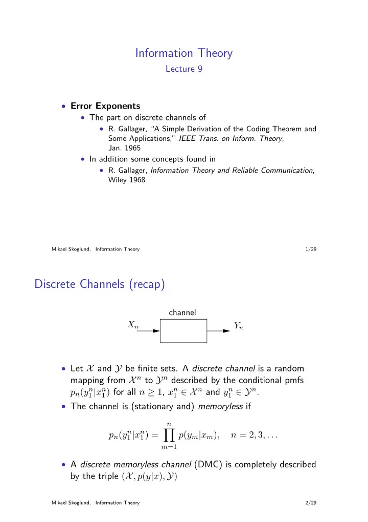
channel Xn Yn

Let X and Y be finite sets. A discrete channel is a random

mapping from X n to Yn described by the conditional pmfs pn(yn

1 |xn 1) for all n ≥ 1, xn 1 ∈ X n and yn 1 ∈ Yn.

The channel is (stationary and) memoryless if

pn(yn

1 |xn 1) = n

m=1

p(ym|xm), n = 2, 3, . . .

A discrete memoryless channel (DMC) is completely described

by the triple (X, p(y|x), Y)

Mikael Skoglund, Information Theory 2/29

SLIDE 2

Block Channel Codes (recap)

channel encoder decoder ω ˆ ω xn

1(ω)

Y n

1

α β

Define an (M, n) block channel code for a DMC

(X, p(y|x), Y) by

1 An index set IM {1, . . . , M} 2 An encoder mapping α : IM → X n. The set

C

xn

1 : xn 1 = α(i), ∀ i ∈ IM

f codewords is called the codebook.

3 A decoder mapping β : Yn → IM, as characterized by the

decoding subsets Yn(i) = {yn

1 ∈ Yn : β(yn 1 ) = i}, i = 1, . . . , M

Mikael Skoglund, Information Theory 3/29

The rate of the code is

R log M n [bits per channel use]

A code is often represented by its codebook only; the decoder

can often be derived from the codebook using a specific rule (joint typicality, maximum a posteriori, maximum likelihood,. . . )

Assume, in the following, that ω ∈ IM is drawn according to

p(m) = Pr(ω = m)

Mikael Skoglund, Information Theory 4/29

SLIDE 3

Error Probabilities (recap)

For a given code
Conditional

Pe,m =

yn

1 ∈(Yn(m))c

pn(yn

1 |xn 1(m))

(= λm in CT)

Maximal

Pe,max = P (n)

e,max = max m Pe,m

= λ(n) in CT
Overall/average/total

Pe = P (n)

e

=

M

m=1

p(m)Pe,m

Mikael Skoglund, Information Theory 5/29

“Random Coding” (recap)

Assume that the M codewords xn

1(m), m = 1, . . . , M, of a

codebook C are drawn independently according to qn(xn

1), xn 1 ∈ X n =

⇒ P(C) = qn

xn

1(1)

· · · qn
xn

1(M)

.
Error probabilities over an ensemble of codes,
Conditional

¯ Pe,m =

C

P(C)Pe,m(C)

Overall/average/total

¯ Pe =

C

P(C)Pe(C)

Note: In addition to C a decoder needs to be specified

Mikael Skoglund, Information Theory 6/29

SLIDE 4

The Channel Coding Theorem (recap)

A rate R is achievable if there exists a sequence of (M, n)

codes, with M = ⌈2nR⌉, such that P (n)

e,max → 0 as n → ∞.

Capacity C is the supremum of all achievable rates.

For a discrete memoryless channel,

C = max

p(x) I(X; Y )

Previous proof (in CT) based on typical sequences =

⇒ limited insight, e.g., into how fast P (n)

e,max → 0 as n → ∞ for

R < C. . .

In fact, for any n > 0,

P (n)

e,max < 4 · 2−nEr(R)

where Er(R) is the random coding exponent

Mikael Skoglund, Information Theory 7/29

Exponential Bounds

A code C(n, R) of length n and rate R
Assume p(m) = M−1, a DMC and consider the average error

probability P (n)

e

= 1 M

M

m=1

Pe,m

Bounds easily extended to P (n)

e,max

Non-zero lower bound may not exist for arbitrary p(m)
Upper-bounds (there exists a code)

P (n)

e

≤ 2−nEmin(R), any n > 0

Lower-bounds (for all codes)

P (n)

e

≥ 2−nEmax(R), as n → ∞

Mikael Skoglund, Information Theory 8/29

SLIDE 5

Reliability Function, Error Exponents

The reliability function of a channel,

E(R) = lim

n→∞

− log P ∗

e (n, R)

n , where P ∗

e (n, R) is the minimum over all codes C(n, R)

Lower bounds to E(R) yield upper bounds to P (n)

e

(as n → ∞)

“random coding” Er(R) and “expurgated” Eex(R) exponents
Upper bounds to E(R) yield lower bounds to P (n)

e

(as n → ∞)

“sphere-packing” Esp(R) and “straight-line” Esl(R)

exponents

Mikael Skoglund, Information Theory 9/29

With Emax = max (Er, Eex) and Emin = min (Esp, Esl)

Emax(R) ≤ E(R) ≤ Emin(R)

The critical rate Rcr is the smallest R in [0, C] such that

Emax(R) = Emin(R) = E(R) for Rcr ≤ R ≤ C;

For R ∈ [Rcr, C) the exponent E(R) > 0 in

P (n)

e

≈ 2−nE(R) as n → ∞ for the best possible existing code is known!

Mikael Skoglund, Information Theory 10/29

SLIDE 6

Decoding Rules

Joint typicality (A(n)

ǫ

jointly typical set) Yn(m) = {yn

1 ∈ Yn : (xn 1(m′), yn 1 ) ∈ A(n) ǫ

⇐ ⇒ m′ = m}

Maximum a posteriori (minimum error probability)

Yn(m) = {yn

1 ∈ Yn : m = argmax m′

Pr(m′|yn

1 )}

Maximum likelihood (a priori unknown / unmeaningful /

uniform) Yn(m) = {yn

1 ∈ Yn : m = argmax m′

pn(yn

1 |xn 1(m′))}

To derive existence results it suffices to consider a specific rule

Mikael Skoglund, Information Theory 11/29

Two Codewords

Two codewords, C = {xn

1(1), xn 1(2)}, and any channel

pn(yn

1 |xn 1)

Assume maximum likelihood decoding,

Yn(1) = {yn

1 ∈ Yn : pn(yn 1 |xn 1(1)) > pn(yn 1 |xn 1(2))}

Hence, for any s ∈ (0, 1) it holds that Pe,1 =

yn

1 ∈Yn(1)c

pn(yn

1 |xn 1(1))

≤

yn

1 ∈Yn(1)c

pn(yn

1 |xn 1(1))1−spn(yn 1 |xn 1(2))s

≤

yn

1 ∈Yn

pn(yn

1 |xn 1(1))1−spn(yn 1 |xn 1(2))s

An equivalent bound applies to Pe,2

Mikael Skoglund, Information Theory 12/29

SLIDE 7

For a memoryless channel we get (with ¯

m = (m mod 2) + 1)

Pe,m ≤

n

i=1
yi∈Y

p(yi|xi(m))1−sp(yi|xi( ¯ m))s =

n

i=1

gn(s), m = 1, 2

For a BSC(ǫ) with two codewords at distance d

Pe,m ≤ min

s∈(0,1) n

i=1

gn(s) =

2
ǫ(1 − ǫ)

d m = 1, 2

⇒ For a “best” pair of codewords (d = n) Pe,m ≤

2
ǫ(1 − ǫ)

n m = 1, 2 ⇒ For a “typical” pair of codewords (d = n/2) Pe,m ≤

2
ǫ(1 − ǫ)

n/2 m = 1, 2

Mikael Skoglund, Information Theory 13/29

Ensemble Average – Two Codewords

Pick a probability assignment qn on X n, and choose M

codewords in C = {xn

1(1), . . . , xn 1(M)} independently;

P(C) =

M

m=1

qn(xn

1(m))

For memoryless channels, we take qn of the form

qn(xn

1) = n

i=1

q1(xi)

Mikael Skoglund, Information Theory 14/29

SLIDE 8

Thus, for m = 1, 2

¯ Pe,m =

xn

1 (1)∈X n

xn

1 (2)∈X n

qn(xn

1(1))qn(xn 1(2))Pe,m

≤

yn

1 ∈Yn

 

xn

1 (1)∈X n

qn(xn

1(1))pn(yn 1 |xn 1(1))1−s

  ×  

xn

1 (2)∈X n

qn(xn

1(2))pn(yn 1 |xn 1(2))s

  Minimum over s ∈ (0, 1) at s = 1/2 = ⇒ ¯ Pe,m ≤

yn

1 ∈Yn

 

xn

1 ∈X n

qn(xn

1)

pn(yn

1 |xn 1)

 

2

Mikael Skoglund, Information Theory 15/29

For a memoryless channel

¯ Pe,m ≤   

y∈Yn
x∈X

q1(x)

p1(y|x)

2  

n

m = 1, 2

In particular, for a BSC(ǫ) with q1(x) = 1/2

¯ Pe,m ≤ 1 2 √ǫ + √ 1 − ǫ 2n m = 1, 2

0.1 0.2 0.3 0.4 0.5 0.2 0.4 0.6 0.8 1

– Solid:

1 2

√ǫ + √1 − ǫ 2 (random) – Dashed:

2
ǫ(1 − ǫ)

1/2 (typical) – Dotted: 2

ǫ(1 − ǫ) (best)

Mikael Skoglund, Information Theory 16/29

SLIDE 9

Alternative Derivation — Still Two Codewords

Examine the ensemble average directly

¯ Pe,1 =

xn

1 (1)∈X n

qn(xn

1(1))

yn

1 ∈Yn

pn(yn

1 |xn 1(1)) Pr(yn 1 ∈ Yn(1)c)

Since the codewords are randomly chosen

Pr(yn

1 ∈ Yn(1)c)

=

xn

1 (2): pn(yn 1 |xn 1 (1))≤pn(yn 1 |xn 1 (2))

qn(xn

1(2))

≤

xn

1 (2)∈X n

qn(xn

1(2))

pn(yn

1 |xn 1(2))

pn(yn

1 |xn 1(1))

s

Substituting this into the first equation yields the result
This method generalizes more easily!

Mikael Skoglund, Information Theory 17/29

Bound on ¯ Pe,m – Many Codewords

As before,

¯ Pe,m =

xn

1 (m)∈X n

qn(xn

1(m))

yn

1 ∈Yn

pn(yn

1 |xn 1(m)) Pr(yn 1 ∈ Yn(m)c)

For M ≥ 2 codewords, any ρ ∈ [0, 1] and s > 0

Pr(yn

1 ∈ Yn(m)c)

≤ Pr(

m′=m

{yn

1 ∈ Yn(m′)})

≤  

m′=m

Pr(yn

1 ∈ Yn(m′))

 

ρ

≤  (M − 1)

xn

1 ∈X n

qn(xn

1)

pn(yn

1 |xn 1)s

pn(yn

1 |xn 1(m))s

 

ρ

Mikael Skoglund, Information Theory 18/29

SLIDE 10

Substitute back into the first equation

¯ Pe,m ≤ (M − 1)ρ

yn

1 ∈Yn

 

xn

1 ∈X n

qn(xn

1)pn(yn 1 |xn 1)s

 

ρ

×  

xn

1 (m)∈X n

qn(xn

1(m))pn(yn 1 |xn 1(m))1−sρ

  Minimize over s > 0 (see HW prob.) = ⇒ ¯ Pe,m ≤ (M − 1)ρ

yn

1 ∈Yn

 

xn

1 ∈X n

qn(xn

1)pn(yn 1 |xn 1)1/(1+ρ)

 

1+ρ

Mikael Skoglund, Information Theory 19/29

For memoryless channels

¯ Pe,m ≤ (M − 1)ρ  

y∈Y

x∈X

q1(x)p1(y|x)1/(1+ρ) 1+ρ 

n

Define

E0(ρ, q1) − log

y∈Y
x∈X

q1(x)p1(y|x)1/(1+ρ) 1+ρ

Using M − 1 < 2nR, we get

¯ Pe,m ≤ 2−n[E0(ρ,q1)−ρR]

Mikael Skoglund, Information Theory 20/29

SLIDE 11

Random Coding Exponent

To minimize the upper-bound on ¯

Pe,m, define the random coding (Gallager) exponent Er(R) = max

ρ,q1 (E0(ρ, q1) − ρR)

Thus, for the ensemble average error probabilities

¯ Pe,m ≤ 2−nEr(R) = ⇒ ¯ P (n)

e

≤ 2−nEr(R)

Since at least one code in the ensemble has error probability

¯ P (n)

e

(or less), there exists a “good” code satisfying P (n)

e

≤ 2−nEr(R)

But, this says nothing about Pe,m!

Mikael Skoglund, Information Theory 21/29

To bound Pe,m take a code with 2M
= 2⌈2nR⌉
codewords,

which satisfies the inequality for equiprobable messages P (n)

e

= 1 2M

2M

m=1

Pe,m ≤ 2−nEr( log 2M

n

)

Throw away the worst M codewords including all that satisfy

Pe,m ≥ 2 · 2−nEr( 1+log M

n

)

Since the decoding subsets didn’t get smaller, the remaining

M codewords satisfy (since ρ ∈ [0, 1]) Pe,m ≤ 2 · 2−nEr(R+ 1

n ) ≤ 2 · 2−n[Er(R)− 1 n]

⇒ There exists at least one code such that for any n > 0 ∀m: Pe,m ≤ 4 · 2−nEr(R) = ⇒ Pe,max ≤ 4 · 2−nEr(R)

Mikael Skoglund, Information Theory 22/29

SLIDE 12

The Coding Theorem Based on Er(R)

Theorem: For any DMC (X, p(y|x), Y) the random coding

exponent Er(R) is a convex, decreasing and positive function

f R for 0 ≤ R < C where

C = max

p(x) I(X; Y )

where I(X; Y ) =

x,y

p(y|x)p(x) log p(y|x) p(y) with p(y) =

x p(y|x)p(x), and where the maximum is over

all possible pmf’s on X.

Mikael Skoglund, Information Theory 23/29

Examples of Er(R)

Binary symmetric channel with crossover probability ǫ

Er(R) =    1 − 2 log √ǫ + √1 − ǫ

− R

R ≤ Rcr d(h−1(1 − R)ǫ) Rcr ≤ R ≤ C C ≤ R where

Rcr = 1 − h

√ǫ

√ǫ+√1−ǫ

(critical rate)

C = 1 − h(ǫ) (capacity) h(ǫ) = −ǫ log ǫ − (1 − ǫ) log(1 − ǫ) (binary entropy) d(δǫ) = δ log δ

ǫ + (1 − δ) log 1−δ 1−ǫ

(binary relative entropy)

Mikael Skoglund, Information Theory 24/29

SLIDE 13

Very noisy channels

p1(y|x) = p(y)(1 + ǫx,y), |ǫx,y| ≪ 1 Using second-order approximation in ǫx,y Er(R) ≈     

C 2 − R

R < C

4

√ C − √ R 2

C 4 ≤ R ≤ C

C ≤ R

Mikael Skoglund, Information Theory 25/29

Some Comments on Other Error Exponents

Expurgated exponent Eex
strengthens Er for small rates
generally agrees with Er on part of its linear portion (R < Rcr)
can be infinite!
Sphere-packing exponent Esp
agrees with Er on its non-linear part (R > Rcr)
can also be infinite!
Straight-line exponent Esl
line through (0, Eex(0)), tangent to Esp (when Eex(0) < ∞)

Mikael Skoglund, Information Theory 26/29

SLIDE 14

Large Deviations Theory. . .

Tight connections to large deviations theory, Chernoff

bounds,. . .

Mikael Skoglund, Information Theory 27/29

A Typical Scenario – BSC(0.05)

curves top-to-bottom
Esp(R)
Eex(R)
Er(R)
marks right-to-left
capacity
critical rate
??

0.2 0.4 0.6 0.8 1 0.2 0.4 0.6 0.8 1 1.2

Mikael Skoglund, Information Theory 28/29

SLIDE 15