Information Theoretic Metric Learning Instructor: Sham Kakade 1 - PDF document

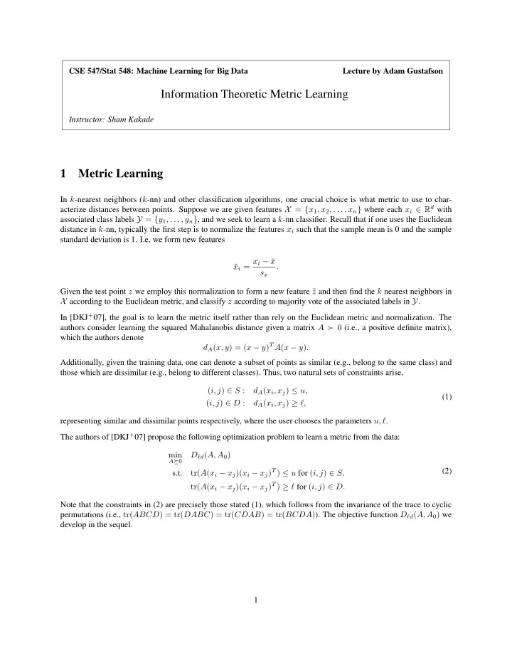
CSE 547/Stat 548: Machine Learning for Big Data Lecture by Adam Gustafson Information Theoretic Metric Learning Instructor: Sham Kakade 1 Metric Learning In k -nearest neighbors ( k -nn) and other classification algorithms, one crucial choice is what metric to use to char- acterize distances between points. Suppose we are given features X = { x 1 , x 2 , . . . , x n } where each x i ∈ R d with associated class labels Y = { y 1 , . . . , y n } , and we seek to learn a k -nn classifier. Recall that if one uses the Euclidean distance in k -nn, typically the first step is to normalize the features x i such that the sample mean is 0 and the sample standard deviation is 1. I.e, we form new features x i = x i − ¯ x ˜ . s x Given the test point z we employ this normalization to form a new feature ˜ z and then find the k nearest neighbors in X according to the Euclidean metric, and classify z according to majority vote of the associated labels in Y . In [DKJ + 07], the goal is to learn the metric itself rather than rely on the Euclidean metric and normalization. The authors consider learning the squared Mahalanobis distance given a matrix A ≻ 0 (i.e., a positive definite matrix), which the authors denote d A ( x, y ) = ( x − y ) T A ( x − y ) . Additionally, given the training data, one can denote a subset of points as similar (e.g., belong to the same class) and those which are dissimilar (e.g., belong to different classes). Thus, two natural sets of constraints arise, ( i, j ) ∈ S : d A ( x i , x j ) ≤ u, (1) ( i, j ) ∈ D : d A ( x i , x j ) ≥ ℓ, representing similar and dissimilar points respectively, where the user chooses the parameters u, ℓ . The authors of [DKJ + 07] propose the following optimization problem to learn a metric from the data: min D ℓd ( A, A 0 ) A � 0 tr( A ( x i − x j )( x i − x j ) T ) ≤ u for ( i, j ) ∈ S, (2) s.t. tr( A ( x i − x j )( x i − x j ) T ) ≥ ℓ for ( i, j ) ∈ D. Note that the constraints in (2) are precisely those stated (1), which follows from the invariance of the trace to cyclic permutations (i.e., tr( ABCD ) = tr( DABC ) = tr( CDAB ) = tr( BCDA ) ). The objective function D ℓd ( A, A 0 ) we develop in the sequel. 1

2 Bregman Divergences 2.1 Definition and Properties Suppose we have a strictly convex, differentiable function φ : R d → R , defined over a convex set Ω = dom( φ ) ⊂ R d . Given such a function, one generalized notion of a distance induced by such a function is as follows: Definition 1 (Bregman Divergence) . The Bregman divergence with respect to φ is a map D φ : Ω × relint(Ω) → R , defined as D φ ( x, y ) = φ ( x ) − φ ( y ) − �∇ φ ( y ) , x − y � , where � x, y � = x T y denotes the usual inner product in R m . Intuitively, it should be clear from the definition that the Bregman divergence measures the error in first order approx- imation of φ ( x ) around y . The Bregman divergence is not a metric in the usual sense. In particular, D φ ( x, y ) � = D φ ( y, x ) in general, and the triangle inequality does not hold. We enumerate some of its properties (verify!): • Non-negativity : D φ ( x, y ) ≥ 0 with equality if and only if x = y . – Follows directly from the first-order condition of strict convexity for the function φ . • Strict Convexity in x : D φ ( x, y ) is strictly convex in its first argument. – Follows directly from the first-order condition of strict convexity for the function φ . • (Positive) Linearity : D a 1 φ 1 + a 2 φ 2 ( x, y ) = a 1 D φ 1 ( x, y ) + a 2 D φ 2 ( x, y ) given a 1 , a 2 > 0 . • Gradient in x : ∇ x D φ ( x, y ) = ∇ φ ( x ) − ∇ φ ( y ) . • Generalized Law of Cosines : D φ ( x, y ) = D φ ( x, z ) + D φ ( z, y ) − �∇ φ ( y ) − ∇ φ ( z ) , x − z � . – Follows directly from the definition. Compare to the law of cosines with in Euclidean spaces: � x − y � 2 2 = � x − z � 2 2 + � z − y � 2 2 − 2 � x − z � 2 � z − y � 2 cos ∠ xzy Here are some examples of some Bregman divergences induced by strictly convex functions: • Mahalanobis Distance : Given A ≻ 0 , let Ω = R d and φ ( x ) = x T Ax . Then D φ ( x, y ) = ( x − y ) T A ( x − y ) . – Euclidean Metric : Letting φ ( x ) = � x � 2 2 results in the Euclidean metric D φ ( x, y ) = � x − y � 2 2 . • Generalized Information Divergence : Let Ω = { x ∈ R d | x i > 0 for all i } . Then φ ( x ) = � d i =1 x i log x i � � implies that D φ ( x, y ) = � d x i log( x i y i ) + ( x i − y i ) . i =1 – Relative Entropy/Kullback-Leibler (KL) Divergence : Additionally require that � x, 1 � = 1 for all x ∈ Ω . Then φ ( x ) = � d i =1 x i log x i results in D φ ( x, y ) = � d i =1 x i log y i x i , the KL divergence between probability mass functions x and y . Finally, we introduce the concept of a Bregman projection onto a convex set. Definition 2 (Bregman Projection) . Given a Bregman Divergence D φ : Ω × relint(Ω) → R , a closed convex set K ⊂ Ω , and a point x ∈ Ω , the Bregman projection of x onto K is the unique ( why? ) point x ⋆ = argmin ˜ x ∈ K D φ (˜ x, x ) . (3) 2

When we consider the function φ ( x ) = � x � 2 2 , note that the Bregman projection corresponds to the orthogonal projec- tion onto a convex set, i.e., x ⋆ = argmin ˜ x − x � 2 x ∈ K � ˜ 2 , (4) so the Bregman projection generalizes the notion of an orthogonal projection. One can show that a generalization of the Pythagorean theorem for such a projection x ⋆ holds. Given any y ∈ K , we have D φ ( x, y ) ≥ D φ ( x, x ⋆ ) + D φ ( x ⋆ , y ) . In the Euclidean case, note that by the law of cosines this implies the angle ∠ xx ⋆ y is obtuse. 2.2 Matrix Bregman Divergences Let S n ⊂ R n × n denote the space of real symmetric matrices. Given a strictly convex, differentiable function φ : S n → R , the Bregman matrix divergence [DT07] is defined as D φ ( A, B ) = φ ( A ) − φ ( B ) − �∇ φ ( B ) , A − B � . Note here that � A, B � = tr( AB ) denotes the inner product on the space of symmetric matrices which induces the Frobenius norm, i.e, � A, A � = � A � 2 F , the sum of the squared entries of A . Usually the function φ will be determined by the composition of an eigenvalue map with another convex function, e.g., φ = ϕ ◦ λ , where λ : S n → R n yields the eigenvalues of a symmetric matrix in decreasing order. 2.2.1 The Log Det (Burg) Divergence and Properties One important example yields the objective function employed in [DKJ + 07]. By taking the Burg entropy of the eigenvalues { λ i } n i =1 of A , we have n n � � φ ( A ) = − log λ i = − log λ i = − log det A, i =1 i =1 which is a strictly convex function with domain of the positive definite cone [BV04]. Using this function yields the so-called “Burg” or “log det” divergence, D ℓd ( A, B ) = tr( AB − 1 ) − log det( AB − 1 ) − n. (5) To see this, note that φ ( A ) − φ ( B ) = − log det( AB − 1 ) , the trace is invariant to cyclic permutations, and ∇ φ ( B ) = − B − 1 . To deduce that ∇ φ ( X ) = − X − 1 , one approach is given in [BV04] is to argue via a first-order approximation as follows. Let Z = X + ∆ X . Then log det Z = log det( X 1 / 2 ( I + X − 1 / 2 ∆ XX − 1 / 2 ) X 1 / 2 ) = log det X + log det( I + X − 1 / 2 ∆ XX − 1 / 2 ) n � = log det X + log(1 + λ i ) , i =1 3