INDIRECT UTILITY FUNCTION U ( P x , P y , M ) = max { U ( x, y ) | - - PDF document

ECO 305 — FALL 2003 — September 25

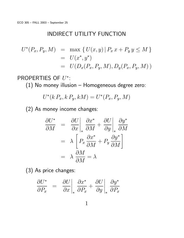
INDIRECT UTILITY FUNCTION U ∗(Px, Py, M) = max { U(x, y) | Px x + Py y ≤ M } = U(x∗, y∗) = U(Dx(Px, Py, M), Dy(Px, Py, M) ) PROPERTIES OF U ∗: (1) No money illusion — Homogeneous degree zero: U ∗(k Px, k Py, kM) = U ∗(Px, Py, M) (2) As money income changes: ∂U ∗ ∂M = ∂U ∂x

¯ ¯ ¯ ¯ ¯

∗

∂x∗ ∂M + ∂U ∂y

¯ ¯ ¯ ¯ ¯

∗

∂y∗ ∂M = λ

"

Px ∂x∗ ∂M + Py ∂y∗ ∂M

#

= λ ∂M ∂M = λ (3) As price changes: ∂U∗ ∂Px = ∂U ∂x

¯ ¯ ¯ ¯ ¯

∗

∂x∗ ∂Px + ∂U ∂y

¯ ¯ ¯ ¯ ¯

∗

∂y∗ ∂Px 1

= λ

"

Px ∂x∗ ∂Px + Py ∂y∗ ∂Px

#

= −λ x∗ (just like M ↓ by x∗) (Last step: differentiate adding-up identity w.r.t. Px: Px x∗ + Py y∗ = M x∗ + Px ∂x∗ ∂Px + Py ∂y∗ ∂Px = 0 ) Divide price- and income-change equations : Roy’s Identity: x∗ = − ∂U∗/∂Px ∂U ∗/∂M (4) Contours of U ∗ in (Px, Py) space with M fixed: (Like theater with stage at NE corner) 2

EXPENDITURE FUNCTION Solve the indirect utility function for income: u = U∗(Px, Py, M) ⇐ ⇒ M = M∗(Px, Py, u) M∗(Px, Py, u) = min { Px x + Py y | U(x, y) ≥ u } “Dual” or mirror image of utility maximization problem. Economics — income compensation for price changes Optimum quantities — Compensated or Hicksian demands x∗ = DH

x (Px, Py, u) ,

y∗ = DH

y (Px, Py, u)

PROPERTIES OF M ∗: (1) Homogeneous degree 1 in (Px, Py) holding u fixed: M ∗(k Px, k Py, u) = k M ∗(Px, Py, u) (2) Hotelling’s or Shepherd’s Lemma — Compensated demands partial derivatives w.r.t. prices: DH

x (Px, Py, u) = ∂M ∗/∂Px , DH y (Px, Py, u) = ∂M ∗/∂Py

Proof: M ∗ = Px DH

x + Py DH y , u = U(DH x , DH y ). So

∂M ∗/∂Px = DH

x + Px ∂DH x /∂Px + Py ∂DH y /∂Px

= Ux ∂DH

x /∂Px + Uy ∂DH y /∂Px

= λ [ Px ∂DH

x /∂Px + Py ∂DH y /∂Px ]

3

(3) “Weakly” concave in (Px, Py) holding u fixed. Cobb-Douglas example: (Px)1/3 (Py)2/3 PROPERTIES OF HICKSIAN DEMAND FUNCTIONS: (1) Own substitution effect negative: ∂x ∂Px

¯ ¯ ¯ ¯ ¯

u=const

= ∂DH

x

∂Px = ∂2M ∗ ∂P 2

x

≤ 0 (2) Symmetry of cross-price effects: ∂DH

x

∂Py = ∂2M∗ ∂Px∂Py = ∂DH

y

∂Px (Net) substitutes if > 0, complements if < 0 General concept : Comparative statics 4

COBB-DOUGLAS EXAMPLE (Direct) UTILITY FUNCTION: U(x, y) = α ln(x) + β ln(y), α + β = 1 x∗ = α M/Px, y∗ = β M/Py INDIRECT UTILITY FUNCTION U∗(Px, Py, M) = α [ln(α) + ln(M) − ln(Px) ] +β [ln(β) + ln(M) − ln(Py) ] = junk + ln(M) − α ln(Px) − β ln(Py) Roy’s Identity: − ∂U∗/∂Px ∂U ∗/∂M = − − α/Px 1/M = α M Px = x∗ EXPENDITURE FUNCTION M∗ = M ∗(Px, Py, u) = eu (Px)α (Py)β Hicksian demand functions xH = α eu (Px)α−1 (Py)β, yH = β eu (Px)α (Py)β−1 5

SLUTSKY EQUATION Link between Marshallian and Hicksian demands Equal if u = U ∗(Px, Py, M), M = M ∗(Px, Py, u). For good i where i may be either x or y, DH

i (Px, Py, u) = DM i (Px, Py, M ∗(Px, Py, u) )

Now let Pj change, where j may be x or y ∂DH

i

∂Pj = ∂DM

i

∂Pj + ∂DM

i

∂M ∂M ∗ ∂Pj = ∂DM

i

∂Pj + ∂DM

i

∂M DH

j

= ∂DM

i

∂Pj + ∂DM

i

∂M DM

j

For example ∂x ∂Py

¯ ¯ ¯ ¯ ¯

u=const

= ∂x ∂Py

¯ ¯ ¯ ¯ ¯

M=const

+ y ∂x ∂M Price derivative of compensated demand = Price derivative of uncompensated demand + Income effect of compensation. If i = j, LHS is negative. Then Giffen implies Inferior 6