Implementing DNNs What this lecture is about: on Embedded - - PDF document

1

Implementing DNNs

• n Embedded

GPU-based Platforms GPU based Platforms

Alessandro Biondi

This lecture

• What this lecture is about:

– Overview of frameworks for implementing DNNs with hardware acceleration on GPU-based embedded platforms – A deep dive into TensorRT, the state-of-the-art framework by Nvidia for efficiently deploying DNNs E l f l t d DNN i f N idi J t TX2

2

– Examples of accelerated DNN inference on Nvidia Jetson TX2

• Warning:

– The second part of this lecture is technical (it’s about programming in C++ with the TensorRT API) and I suppose you have a basic knowledge of C++11 – Code is simplified to fit in the slides, but quite close to the real one – Anyway, you’ll see real code in the demos at the end of this lecture

This lecture

• What this lecture is not about:

– You won’t see new models for DNNs – You won’t learn anything related to the internal structure of DNNs – You won’t see how to train DNNs and to manage datasets: l th i f h i dd d

3

• nly the inference phase is addressed

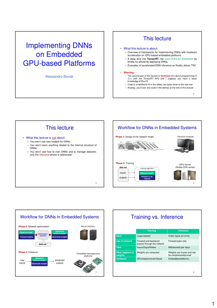
Workflow for DNNs in Embedded Systems

Phase 1: Design of the network model

Personal computer

4 Network model

inputs

• utputs

Weights to be trained training algorithm

data set

GPU server (Nvidia DGX series) Phase 2: Training Phase 3: Network optimization

Server machine

Network model Trained weights Optimized network model Optimized weights

Optimization algorithm

Workflow for DNNs in Embedded Systems

5

data set

Phase 4: Inference

Optimized network model Optimized weights

new inputs predicted

• utputs

Embedded heterogeneous platforms

Training vs. Inference

Training Inference Input Large dataset A few inputs at a time Use of network Forward and backward th h th t k Forward pass only

6

passes through the network Time Hours/Days/Weeks Milliseconds per input What happens to weights Weights are computed Weights are known and can be compressed/pruned Hardware GPU-based server/Cloud Embedded platforms

2

Landscape of Embedded Het. Platforms

7

Embedded GPUs

This lecture

8

Data from connecttech.com

Nvidia Jetson TX2

Jetson TX2 module

9

Embedded GPUs: performance

DNN 10 Data from nvidia.com

Jetson TX2 Module

11 Figure from nvidia.com

Tegra X2

Main CPUs (ARMv8) - asymmetric

12 Figure from nvidia.com

GPU

3

JetPack

• Nvidia JetPack SDK is a comprehensive resource for

building AI applications

• JetPack bundles all of the Jetson platform software

– accelerated software libraries, APIs, sample applications, developer tools, and documentation

• and includes the Nvidia Jetson Linux Driver Package

13

• …and includes the Nvidia Jetson Linux Driver Package

(L4T).

– L4T provides the Linux kernel, bootloader, NVIDIA drivers, flashing utilities, sample filesystem, and more for the Jetson platform.

DNNs on GPUs

• DNNs on GPUs can be deployed by:

– Implementing layers from scratch with CUDA (unrealistic for modern DNNs, it’s like re-inventing the wheel) – Using cuBLAS – Using cuDNN

14

– Using standard DNN frameworks (TensorFlow, Caffe, …) (internally, they leverage cuBLAS or cuDNN) – Using TensorRT (state-of-the-art for high-performance inference)

CUDA

• CUDA is a parallel computing platform and programming model

that makes using a GPU for general purpose computing simple and elegant.

• The developer still programs in C/C++ (also other widespread

languages are supported).

• CUDA incorporates extensions of these languages in the form of

15

a few basic keywords.

cuBLAS

• Basic

Linear Algebra Subprograms (BLAS) is a specification that prescribes a set of low-level routines for performing common linear algebra operations

– De-facto standard low-level routines for linear algebra

• The

NVIDIA cuBLAS library is a fast GPU-accelerated implementation of the standard basic linear algebra subroutines

16

implementation of the standard basic linear algebra subroutines (BLAS).

• Using cuBLAS APIs, you can speed up your applications by

deploying compute-intensive operations to a single GPU or scale up and distribute work across multi-GPU configurations efficiently. https://developer.nvidia.com/cublas

cuDNN

• cuDNN

by Nvidia is a GPU-accelerated library

• f

primitives for deep neural networks.

• cuDNN

provides highly tuned implementations for standard routines such as forward and backward convolution, pooling, normalization, and activation layers.

17

• Deep learning researchers and framework developers

worldwide rely on cuDNN for high-performance GPU acceleration.

– It allows them to focus on training neural networks and developing software applications rather than spending time

• n low-level GPU performance tuning.

https://developer.nvidia.com/cudnn

cuDNN

Speed-up for training ImageNet with Caffe (on a standard dataset)

18 Source: gigaom.com

4

GPU Support in DNN Frameworks

• Most

(if not all) DNN frameworks, such as TensorFlow and Caffe, dispose of a built-in support for Nvidia GPUs

• The support consists in implementations of DNN

layers with cuBLAS and cuDNN

19

y

tf.device('/device:GPU:0')

TensorFlow (python API) Caffe (python API)

caffe.set_mode_gpu()

TensorRT TensorRT

TensorRT

• TensorRT

is a framework that facilitates high performance inference

• n

NVIDIA graphics processing units (GPUs).

• TensorRT takes a trained network which consists of

21

TensorRT takes a trained network, which consists of a network definition and a set of trained parameters, and produces a highly optimized runtime engine which performs inference for that network. Intro, generalities, etc.

• It’s built upon cuDNN

TensorRT: performance

• Up to 140x in throughput (images per sec) on Nvidia

Tesla v100 w.r.t. CPUs

22 Image from nvidia.com

Using TensorRT

23 Image from nvidia.com

Using TensorRT

• Step 1: Optimize trained networks with TensorRT Optimizer

24

• Step 2: Deploy optimized networks with TensorRT Runtime Engine

Images from nvidia.com

TensorRT

5

Using TensorRT

• TensorRT inputs the DNN model and the corresponding weights

(trained network)

• The input can be provided with a custom API or by loading files

exported by DNN frameworks such as Caffe and TensorFlow

25

DNN Model

DNN Weights

TensorRT GPGPU

Internally uses CUDA (cuDNN) to execute on GPUs (not exposed to users)

Using TensorRT

26 Image from nvidia.com

TensorRT: optimizations

TensorRT performs four types of optimizations: – Weight quantization and precision calibration – Layer and tensor fusion – Kernel auto-tuning D i t

27

– Dynamic tensor memory

Quantized DNNs

• The performance of modern DNNs is impressive but

they require to perform heavy computations that involve a huge set of parameters (weights, activations, etc.)

– In particular, the convolution

• perations

are very computationally intensive!

28

• Such computations may be unsuitable for resource-

constrained platforms such as those that are typically available in embedded systems

– Inference may be very slow on an embedded platform violating timing constraints – They also consume a lot of energy

Quantized DNNs

• The research of quantized DNNs has attracted a lot
• f

attention from the deep learning community in recent years

• The goal of quantization is to contain the memory

footprint of trained DNNs to achieve faster inference

29

p while not significantly penalizing the network accuracy

• Joint

solutions from machine learning, numerical

• ptimization, and computer architectures are required

to achieve this goal

• Y. Guo, “A Survey on Methods and Theories of Quantized Neural Networks”,

arXiv:1808.04752v2

Quantized DNNs

• Standard

DNNs come with 32-bit floating points parameters and hence require floating-point units (FPU) to perform the corresponding computations

• Conversely, the operations required to infer a quantized

neural networks (e.g., with integer parameters) are

30

( g , g p ) typically bitwise operations that can be carried out by arithmetic logic units (ALU)

– ALU are faster than FPU and consume much less energy!

6

Quantized DNNs

• Quantization typically reduces the precision of the

weights and hence also their footprint

– Example: from 32-bit floating point (FP32) numbers to 8-bit integer (INT8) numbers with uniform quantization

range of values for the weight 31 min max g g min max example of quantized weight with INT8 precision range split in 256 intervals

Binarized DNNs

• An extreme quantization scheme for DNNs consists

in using binary parameters

• A possible (and typical) way to perform binarization

is to adopt the sign function to the original weights and then encode ‘+1’ and ‘-1’ with the two states allowed by a single bit

32

allowed by a single bit

• Binarized DNNs can achieve an accuracy of 98.8%

in recognizing characters from the MNIST dataset!

Courbariaux et al., “Binaryconnect: Training deep neural networks with binary weights during propagations”, Advances in Neural Information Processing Systems 2015

Binarized DNNs

• The dot product of two binary vectors a and b can be

computed as bitcount(a and b), where bitcount counts the number of 1s of a binary vector

1 1 1 1

33

1 1 1 1 1 1 1 1 1 1

= 1x0 + 1x0 + 0x1 + 1x1 + 0x1 + 1x1 + 0x1 + 1x1 = 3

X

1 1 1 1 1 1 1 1 1 1

AND =

1 1 1

bitcount(…) = 3

Quantization methods

The quantization methods proposed to date can be divided into two classes:

• Deterministic quantization

– Rounding

34

g – Clustering – Rounding with calibration – Quantization as optimization – …

• Stochastic quantization

– Random rounding – Probabilistic quantization – …

Quantization methods: rounding

35

with

Quantization methods: rounding

36

with

0.1 0.2 0.3 0.4 0.5 0.6 0.7 0.8 0.9 0.0 1.0 1 2 3 4 5 6 7 8 9 Example with s=10 max min discrete domain continuous domain

7 Quantization methods: rounding

• PROs

– Easy and lightweight method to perform quantization

• CONs

It has been found that the network performance may drop

37

– It has been found that the network performance may drop dramatically after each rounding operation – To achieve better performance the rounding should be performed during training

• Both real and quantized values must be stored during training, hence

increasing the memory footprint

• It is harder for the training process to converge when using quantized

values

Quantization methods: clustering

• The weights are first clustered into K clusters with a k-means

algorithm – Clusters are formed such that the distance of the weights in each cluster to the centroid of the cluster is minimized:

38

• The weights of each cluster are then replaced by the centroid of

the cluster

– An integer encoding of the weights can be used just to store the cluster id

• In 2014, Gong et al. showed that this approach allows

achieving a compression factor from 16x to 24x with 1% accuracy loss on the ImageNet dataset (w.r.t. to state-of-the-art

DNNs in 2014)

• PROs

– Tends to achieve better performance w.r.t. rounding – Can be easily applied to pre-trained networks

• CONs

Quantization methods: clustering

39

• CONs

– Due to the large number of weights (tents of millions on a state-of- the-art network), k-means clustering is very computationally intensive

Quantization methods: rounding with calibration

• The key goal of quantization is to minimize information loss
• Note that the weights of a network are not arbitrary but tend to

follow some distribution

– This observation can be leveraged to select the quantized values

40 Histogram of weight values of LeNet-5 after training on MNIST. The blue line is the fitted Gaussian distribution. (from Guo’s survey)

Quantization methods: rounding with calibration

• Information loss due to quantization can be measured with

respect to a calibration data set

• Also

the value

• f

activation functions will follow some distribution, which can be recorded on the calibration data set

41

Image from Szymon Migacz’s presentation, Nvidia, 2017

Quantization methods: rounding with calibration

Calibration algorithm

• Inputs:

– Network trained with floating-point weights – Calibration dataset

42

• Steps:
• 1. Run inference with floating-point weights on calibration dataset
• 2. Collect histograms of activations
• 3. Generate several quantized distributions for the weights and

select the one that minimizes information loss

• 4. Quantize weights accordingly
• Outputs:

– Network with quantized weights

8

• PROs

– Can be easily applied to pre-trained networks – Quantization is not particularly computationally expensive (~minutes on a desktop workstation) – Allows achieving very low accuracy loss

Quantization methods: rounding with calibration

43

Allows achieving very low accuracy loss

• CONs

– Performance depends on the calibration data set TensorRT uses rounding with calibration to support quantization

• f DNNs with 8-bit integer (INT8) weights

TensorRT: weights precision

dataset-dependent! 44

Precision calibration for INT8 inference:

• Minimizes

information loss between FP32 and INT8 inference

• n

a calibration dataset

• Completely automatic

Images from nvidia.com

TensorRT: INT8 calibration

• Inputs:

– Network trained with FP32 weights – Calibration dataset

• TensorRT will:

R i f i FP32 lib ti d t t

45

– Run inference in FP32 on calibration dataset – Collect statistics – Run calibration algorithm  optimal scaling factors – Quantize FP32 weights to INT8

TensorRT: INT8 calibration

46

…calibration of the weights precision is an active research topic! Let us know if you’re interested…

Image from Szymon Migacz’s presentation, Nvidia, 2017

TensorRT: INT8 calibration

Accuracy performance

47 Source: Shashank Prasanna, “Deep Learning Deployment with Nvidia TensorRT”

TensorRT: layer fusion

Non-optimized DNN DNN optimized by TensorRT

Vertical layer fusion

48 Image from nvidia.com

CBR = Convolution, Bias and ReLU

9

TensorRT: layer fusion

Non-optimized DNN DNN optimized by TensorRT

Vertical and horizontal layer fusion

49 Image from nvidia.com

CBR = Convolution, Bias and ReLU

TensorRT: layer fusion

50 Source: Shashank Prasanna, “Deep Learning Deployment with Nvidia TensorRT”

This Lecture

• The next slides are about how to use the C++ API of

TensorRT by taking in input a DNN modeled with Caffe

• You’ll

see that implementing high-performance inference is not straightforward even with mature

51

g tools like TensorRT

Caffe Models

• Caffe networks are distributed with two files

.prototxt .caffemodel

52

Architectural model of the network expressed with Google’s Protocol Buffers Weights of the network The file extension is misleading (don’t ask me why…)

Caffe Models

• “DNNs are compositional models that are naturally

represented as a collection of inter-connected layers that work on chunks of data”

• Layer = Fundamental unit of computation. Layers

convolve filters pool take inner products apply

53

convolve filters, pool, take inner products, apply nonlinearities like rectified-linear and sigmoid, compute losses, etc.

• Blob = Wrapper of the actual data being processed

and passed along the network by Caffe. It’s a standard array and unified memory interface for the framework.

Caffe Layers

• A layer takes input through bottom connections and

makes output through top connections

• Each layer is characterized by

– a name – a type

54

yp – bottom and top blobs – layer-specific parameters

layer { name: “conv1" type: “Convolution" top: “conv1” bottom: “data” }

layer in .prototxt file

10

Caffe Networks

• The network is a set of layers connected in a directed

acyclic graph (DAG)

• Each node of the DAG is a layer, while each edge is

associated to a blob

• A typical net begins with a

data layer that loads from disk and ends with a loss layer that computes the objective for a task such as classification or reconstruction

55

Caffe Networks

56 Image from panderson.me

Caffe Models

• Alternatively to data layers, Caffe models can come

with a special blob to denote the network input

• This blob is specified in the header of the network

description (.prototxt file)

57

name: “ResNet-18” input: “data” input_dim: 1 input_dim: 3 input_dim: 368 input_dim: 640

header of .prototxt file

Visualizing Caffe Networks

• A nice tool is available to visualize Caffe Networks

http://ethereon.github.io/netscope/ quickstart.html

58