Frameworks for DNNs DNNs are typically developed, trained, and - - PDF document

SLIDE 1

3/18/2020 1

Frameworks for DNNs

DNNs are typically developed, trained, and inferred by means

• f specific frameworks (i.e., toolkits, libraries), because they
• provide a simple high-level interface (mostly in Python);
• simplify the creation of new DNNs using a large set of

pre implemented layers (e g convolutions); pre-implemented layers (e.g., convolutions);

• allow training and inferring DNNs on different devices (e.g.,

CPUs, GPUs, mobile) by changing a few lines of code;

• exploit frequent library updates with new features;

In addition, a lot of examples and pre-trained networks are available online.

2

Frameworks for DNNs

The deep learning landscape is constantly changing, hence many frameworks have been developed during the last years, most of them open source: Different frameworks have different features, hence no one is the best for all the problems. Let’s consider some of them.

3

Frameworks for DNNs

• The first widely adopted framework.
• Created in 2007 at the Montreal Institute for Learning

Algorithms (MILA), headed by Yoshua Bengio, one of the i f d l i pioneers of deep learning.

• Developed in Python.
• Can run DNNs on either CPU or GPU architectures.
• Since 2017, it is no longer maintained, due to the release of

many other frameworks, developed by large companies.

4

Frameworks for DNNs

(2013) by UC Berkeley (2015) by Google (2015) by Amazon (2016) (Computational Network Toolkit) by (2016) (Computational Network Toolkit) by

• Microsoft. Now called Microsoft Cognitive Toolkit.

(2017) by Facebook as an evolution of Caffe. (2017) by Facebook. Caffe2 and Pytorch are going to be integrated into a single platform. (2017) (Deep Learning for Java) by Skymind as a deep learning library for Java and Scala.

5

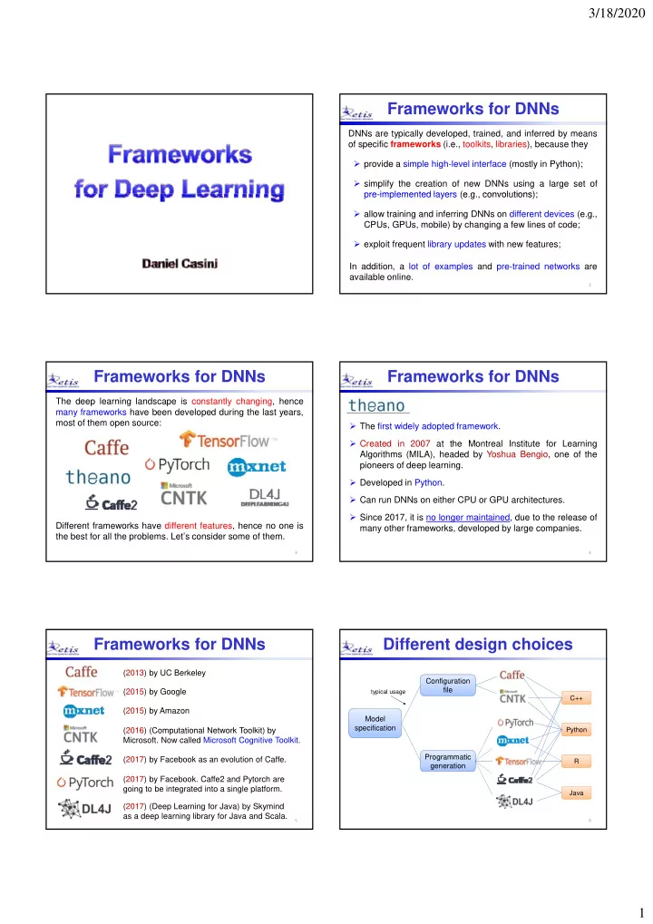
Different design choices

Model specification Configuration file

Python C++

typical usage

6

specification Programmatic generation

Python Java R

SLIDE 2

3/18/2020 2

High-level APIs

Besides these frameworks, there are also high-level interfaces that are wrapped around one or multiple frameworks.

• Released in 2016 by François Chollet (Google).

7

• Python-based library for fast experimentation with DNN.
• It runs on top of TensorFlow, CNTK, Theano, or PlaidML.
• User-friendly, modular, and extensible.
• Quote: "API designed for human beings, not machines".
• It

allows creating a DNN by stacking layers without specifying math operations, but only layer types.

High-level APIs

• Released in 2017 by Amazon and supported by Microsoft.
• High-level Python deep learning interface
• It wraps MXNet and soon it will also include CNTK

8

• It wraps MXNet and soon it will also include CNTK.
• Gluon is a direct competitor for Keras.
• Released in 2017 by Google’s DeepMind.
• It is built on top of TensorFlow.

High-level APIs

• In

2017, Microsoft, Amazon, Facebook, and

• thers

launched ONNX, an Open Neural Network Exchange format to represent deep learning models and port them between different frameworks Open Neural Network Exchange

9

between different frameworks.

• ONNX enables models to be trained in one framework and

transferred to another for inference.

• ONNX supports Caffe2, CNTK, MXNet, PyTorch, and

TensorFlow.

Open source deep learning frameworks (2017)

Frameworks at a glance

10

Facebook Microsoft Google Microsoft Amazon

The complete stack

Keras Gluon ONNX DNN High‐level APIs Appl. Mid l l

11

Python C++ Java

  

CPU GPU TPU

Windows Linux Android iOS

  

Theano Caffe Tensor Flow PyTorch CNTK MXNet

  

DSP HW OS Language Mid‐level APIs

Popularity

TensorFlow s

GitHub users can “star” a repository to indicate that they like it. So GitHub Stars can measure how popular a project is.

Caffe PyTorch CNTK MXNet GitHubStars

12

SLIDE 3

3/18/2020 3

Combined metrics

Power score computed by mixing several criteria, as articles, books, citations, Github activities, Google search volume, etc. Power score 2018

13

At the moment, TensorFlow is the most used framework, followed by Caffe and PyTorch. Main features

Released in 2015 by Google

14

Large community and support TensorBoard visualization tool Scalability to many platforms Good library mgmt and updates Not so intuitive interface Slower than other frameworks

Mid-level TF APIs High-level TF APIs

Layers Datasets Losses Estimators Keras TF learn Metrics TF-sim

The TensorFlow Stack

     

Hardware Operating Systems TensorFlow Distributed Execution Engine Python Frontend C++ TF runtime Language

15

CPU GPU TPU

Windows Linux Android iOS

     

DSP Main features Excellent for CNNs for image processing.

Convolution Architecture For Feature Extraction

Released in 2013 by UC Berkeley

While in TF the network is created by programming, in Caffe layers are created by specifying a set of parameters. Quite fast compared to other frameworks. Command line, Python, C++, and MatLab interface. Not so easy to learn. Not so good with recurrent neural networks and sequence models.

16

Main features Support for dynamic graphs. This is efficient when the input varies, as in text processing. Interactive debugging. Released in 2017 by Facebook

In 2017, TensorFlow introduced Eager Execution, to evaluate

• perations immediately without

gg g Easier to get started. Blend of high-level and low-level APIs. Limited documentation. No graphic visualization tools. No support for Windows (only Linux and macOS).

17

• perations immediately, without

building graphs.

Comparing frameworks

Theano Tensor- Flow Pytorch

Languages Tutorial Material CNN modeling RNN modeling Easy-to-use API Speed Multiple GPU support Keras compatible Python, C++ Python, C++ Python, C++

++ +++ + +++ +++ ++ ++ ++ ++ + +++ ++ +++ ++ ++

NO YES YES YES NO YES

18

Pytorch Caffe MXNet CNTK DL4J

C++ Python, C++ Python, R, Julia, Scala Python, C++ Java, Scala

+ + ++ + +++ +++ +++ ++ + +++ ++ + +++ +++ ++ + ++ + ++ +++ ++ ++ + ++

YES YES YES YES YES NO NO YES YES YES NO

SLIDE 4

3/18/2020 4

NVIDIA framework

Theano Caffe P Torch

DNN Appl. Mid‐level NVIDIA also provides support for DNN development, but only

• n top of their GPU platforms:

19

GPU CUDA

Theano Caffe PyTorch

HW Language APIs Optimiz. Libraries

cuDNN cuBLAS

20

Data Set Finders

There are a lot of data sets on the internet for training DNNs.

• Kaggle: www.kaggle.com

The following are general data set repositories that allow searching for the one you need:

21

• UCI Machine Learning Repository: mlr.cs.umass.edu/ml
• VisualData: www.visualdata.io
• CMU Library: guides.library.cmu.edu/machine-learning/datasets

Data sets are usually divided into categories.

Data sets

Natural images

• MNIST: handwritten digits (yann.lecun.com/exdb/mnist/).
• CIFAR10 / CIFAR100: 32×32 image dataset with 10 / 100 categories

(www.cs.utoronto.ca/~kriz/cifar.html).

• COCO: large dataset for object detection, segmentation, and captioning

(cocodataset org)

22

(cocodataset.org).

• ImageNet: large image database organized according to the WordNet

hierarchy (www.image-net.org).

• Pascal VOC: dataset for image classification, object detection, and

segmentation (https://pjreddie.com/projects/pascal-voc-dataset-mirror/).

• COIL 20: 128×128 images of 20 objects taken at different rotation angles

(www.cs.columbia.edu/CAVE/software/softlib/coil-20.php).

• COIL100: 128×128 images of 100 objects taken at different rotation

angles (www1.cs.columbia.edu/CAVE/software/softlib/coil-100.php).

Faces

• Labelled Faces in the Wild: 13,000 images of faces collected from the

web, labelled with the person name (vis-www.cs.umass.edu/lfw).

• Olivetti:

images

• f

several people faces at different angles (www.cs.nyu.edu/~roweis/data.html).

• Sheffield: 564 images of 20 individuals each shown in a range of poses

Data sets

23

Sheffield: 564 images of 20 individuals each shown in a range of poses (https://www.sheffield.ac.uk/eee/research/iel/research/face).

Text

• 20 newsgroups: Classification task to map word occurrences into 20

newsgroup IDs (qwone.com/~jason/20Newsgroups).

• Penn Treebank: used for next word prediction or next character prediction

(corochann.com/penn-tree-bank-ptb-dataset-introduction-1456.html).

• Broadcast News: large text dataset used for next word prediction

(https://github.com/cyrta/broadcast-news-videos-dataset).

Speech

• TIMIT Speech Corpus: DARPA Acoustic-Phonetic Continuous Speech

Corpus for phoneme classification (github.com/philipperemy/timit).

• Aurora: Timit with noise and additional information (aurora.hsnr.de).

Data sets

Music

24

• Piano-midi.de: classical piano pieces (www.piano-midi.de).
• Nottingham: over 1000 folk tunes (abc.sourceforge.net/NMD).
• MuseData: a collection of classical music scores (musedata.stanford.edu).
• JSB

Chorales: a dataset

• f

four-part harmonized chorales (https://github.com/czhuang/JSB-Chorales-dataset).

• FMA: a dataset For Music Analysis (github.com/mdeff/fma).

SLIDE 5

3/18/2020 5

MNIST

MNIST is the most popular datasets of handwritten digits. It contains a training set of 60,000 examples and a test set of 10,000 examples.

25

Size: 28 x 28 Greylevels: 256 (0  black, 1  white) Label: 0, 1, …, 9

train[i][0] or test[i][0]: i-th example train[i][1] or test[i][1]: i-th label

CIFAR-10

CIFAR-10 consists of 60,000 32x32 color images organized in 10 classes (6,000 images per class). There are 50,000 training images and 10,000 test images:

airplane automobile bi d

26

bird cat deer dog frog horse ship truck

  

COCO

COCO is a large-scale and rich dataset for object detection, segmentation, and captioning.

27

• 330,000 images
• 1.5 million object instances
• 80 object categories
• 91 stuff categories
• 5 captions per image
• 250,000 people with keypoints

Olivetti Faces

Olivetti Faces is a dataset containing 400 images of faces of several people at different angles.

28

• Number of images: 400
• Image size: 64x64
• Color depth: 8 bit, grayscale [0-255]

TensorFlow and Keras

First of all, it must be clarified that:

• Keras is an open-source machine learning library that

generates code for TensorFlow and other frameworks;

• Since 2017, the Keras API is integrated in TensorFlow and

can be used as tf.keras (in a Python environment)

30

• So neural networks can be developed either under Keras or

TensorFlow, using the high level API provided by tf.keras:

SLIDE 6

3/18/2020 6

Installing TF using Pip

TensorFlow and Keras may be installed by using Pip, the package manager of Python. Pip is automatically installed when installing Python. Installation procedure

1. Download and install Python for Windows / Linux / Mac OS from

31

https://www.python.org/downloads/ 2. Open a terminal and issue the commands: C:\User> Python3 ‐m pip install ‐‐upgrade https://storage.googleapis.com/tensorflow/mac/cpu/tensorflow ‐1.12.0‐py3‐none‐any.whl C:\User> pip install tensorflow C:\User> pip install keras

https://www.tensorflow.org/install/pip?lang=python3

Installing Anaconda

Another way to install TensorFlow and Keras is by leveraging Anaconda, an open-source platform developed to perform machine learning in Python on Windows, Linux, and Mac OS. Installation procedure

1. Download Anaconda for Windows / Linux / Mac OS from

32

https://www.anaconda.com/ 2. Install Anaconda 3. Open Anaconda and create a new environment (e.g., neural) 4. From the environment, open a terminal. You should get a prompt like: (neural) C:\User>

To close the terminal type exit.

Installing packages

To use TensorFlow, Keras, and display some plots, we first have to install the following packages:

(neural) C:\User> conda install tensorflow –y (neural) C:\User> conda install keras –y (neural) C:\User> conda install matplotlib –y

33

Notes

• This operation has to be done only once! If you close the terminal and

reopen it later, the packages do not have to be reinstalled.

• Each package may install a number of other packages. For example,

TensorFlow also installs numpy, tensorboard, protobuf, etc.

The list of the packages currently installed in the environment can be seen by the command:

(neural) C:\User> conda list

Practice with Python

If you are not familiar with Python, practice with it first. Here are some useful links: Official materials

• Tutorial:

http://docs.python.org/tutorial/

• Docs:

http://docs.python.org/index.html

34

Books

• Fundamentals of Programming Python (Richard L. Halterman)

https://python.cs.southern.edu/pythonbook/pythonbook.pdf

• A Practical Introduction to Python Programming (Brian Heinold)

https://www.brianheinold.net/python/python_book.html

Slides

• http://tdc-www.harvard.edu/Python.pdf
• https://www.seas.upenn.edu/~cis391/Lectures/python-tutorial.pdf

A look at the MNIST dataset

(neural) C:\User> python >>> from keras.datasets import mnist >>> (x_train, y_train), (x_test, y_test) = mnist.load_data() >>> print(x_train.ndim) dimensions (# of axis of the tensor)

Now, open Python and execute the following commands:

35

3 >>> print(x_train.shape) (60000, 28, 28) >>> print(x_train.dtype) uint8 ( ) It is a 3D tensor # of elements for each axis (60000 images of 28x28 pixels) 8-bit unsigned integer

Displaying the 2nd digit

>>> import matplotlib.pyplot as plt >>> digit = train_images[1] >>> plt.imshow(digit, cmap=plt.cm.binary) >>> plt.show()

36

SLIDE 7

3/18/2020 7

A 3-layer perceptron

128 10

Suppose we want to create a 3-layer network for handwritten digits recognition with the following features:

• Input layer: 28 x 28 images

(i.e., 784 input values);

• Hidden layer: 128 neurons

with ReLU activation function;

38

  

softmax ReLU 28 28

with ReLU activation function;

• Output layer: 10 neurons

with softmax activation function.

Workflow

Once the all the packages have been installed, a neural network can be executed through the following steps:

• 1. Import libraries and modules;
• 2. Import the dataset;

3 P th i t d t d l l b l

• 3. Preprocess the input data and class labels;
• 4. Define the network;
• 5. Compile the network;
• 6. Train the network with the training set;
• 7. Test the network with the test set.

39

Import libraries & data

# import libraries import numpy as np # array library # import the MNIST dataset from keras.datasets import mnist

40

# load the dataset (train_images, train_labels), (test_images, test_labels) = \ mnist.load_data()

Note: the backslash is used to break a line when the text is not between parentheses.

Preprocess data

#reshape data into a 2D array train_images = train_images.reshape((60000, 28*28)) test_images = test_images.reshape((10000, 28*28)) #scale data to 32-bit floats in [0,1] train images = train images .astype('float32') / 255

41

train_images train_images .astype( float32 ) / 255 test_images = test_images.astype('float32') / 255 #convert labels to one-hot encoding from keras.utils import to_categorical train_labels = to_categorical(train_labels) test_labels = to_categorical(test_labels)

One-hot encoding

Sample Category 1 Car 2 Semaphore 3 Person

• A one‐hot encoder performs binarization of the categories and includes

it as a feature to train the model

42

4 Car Sample Car Semaphore Person 1 1 2 1 3 1 4 1

SLIDE 8

3/18/2020 8

Define the network

To define the network, we first import the Sequential model and the Dense layer, and then create the network:

#import the needed model and layer types from keras.models import Sequential from keras.layers import Dense

43

#define the network as a sequence of layers model = Sequential([ Dense(128, activation=‘relu’, input_dim=(28*28)), Dense(10, activation='softmax'), ])

Define the network

Note that the layers can also be added with the .add() method:

model = Sequential() model.add(Dense(128, activation='relu', input_dim=(28*28))) model.add(Dense(10, activation='softmax'))

44

model = Sequential() model.add(Dense(128, input_dim=(28*28))) model.add(Activation('relu')) model.add(Dense(10)) model.add(Activation('softmax'))

As an alternative, the activation function can also be specified as a layer:

Compile the network

To compile the network, we need to specify three more things:

• A loss function to evaluate the error on the training data

(e.g., the mean squared error);

• An optimizer, i.e., the mechanism through which the

network updates its weights (e.g., stochastic gradient descent);

45

model.compile( loss='categorical_crossentropy',

• ptimizer=‘rmsprop',

metrics=['accuracy'])

• A metrics to evaluate the network performance during

training and testing (e.g., the accuracy).

Available Loss functions

There are many loss functions in Keras. Here are a few examples:

• ‘mean_squared_error’
• ‘mean_absolute_error’
• ‘categorical_crossentropy’

46

• ‘binary_crossentropy’
• ‘cosine_proximity’

Available optimizers

A number of optimizers can be specified in Keras:

• SGD (stochastic gradient descent) includes support for learning rate

decay, momentum, and Nesterov momentum.

• Adagrad (Adaptive gradient). It is a modified version of SGD with

multiple learning rates, which are adapted during training.

• RMSProp (Root Mean Square Propogation) It is good for RNNs

47

• RMSProp (Root Mean Square Propogation). It is good for RNNs.
• Adadelta. It is a more robust extension of Adagrad.
• Adam (Adaptive Moment Estimation). It improves RMSProp by using

running averages of gradients and second moments of the gradients.

• Adamax. A variant of Adam based on the infinity norm.
• Nadam

(Nesterov-accelerated Adam). It combines Adam and Nesterov-accelerated SGD.

Compile the network

from keras import optimizers sgd = optimizers.SGD(lr=0.1, decay=1e-6, t 0 9

Other optimizer-specific parameters can be set as follows:

48

momentum=0.9, nesterov=True) model.compile( loss='categorical_crossentropy',

• ptimizer=sgd,

metrics=['accuracy'])

SLIDE 9

3/18/2020 9

Train the network

model.fit(train_images, train_labels, epochs=5, batch_size=128) The network can be trained by calling the .fit() method:

• epochs = # of iterations over the entire data set
• batch_size = # of samples per gradient update

49

Two quantities are displayed during training:

• the loss of the network over the training data
• the accuracy of the network over the training data.

Epoch 1/5 60000/60000 [==============================] ‐ 9s ‐ loss: 0.2524 ‐ acc: 0.9273 Epoch 2/5 51328/60000 [========================>.....] ‐ ETA: 1s ‐ loss: 0.1035 ‐ acc: 0.9692

ETA (estimated time of arrival) is the estimated time to complete one epoch.

Test the network

test_loss, test_acc = model.evaluate(test_images, test_labels) print(‘Test accuracy:', test_acc)

Once training is over, we can check how the network performs

• n the test set by the .evaluate() method:

50

For more information on Keras functions and parameters visit: https://keras.io/

Display graphs

import matplotlib.pyplot as plt history = model.fit(train_images, train_labels, epochs=5, batch_size=128, verbose=0, validation_data=(test_images, test_labels))

A graph of loss and accuracy can be obtained as follows:

51

test_loss, test_acc = model.evaluate(test_images, test_labels) # Get training and validation loss histories train_loss = history.history['loss'] valid_loss = history.history['val_loss'] # Get training and validation accuracy histories train_acc = history.history['acc'] valid_acc = history.history['val_acc']

Display the loss

# Create count of the number of epochs epoch_count = range(1, len(train_loss) + 1) # plot the training and validation loss plt.plot(epoch count, train loss, ‘b-')

A graphical display of the loss can be obtained as follows:

52

plt.plot(epoch_count, train_loss, b ) plt.plot(epoch_count, valid_loss, ‘g-') plt.title(‘model loss') plt.xlabel(‘epoch') plt.ylabel(‘loss') plt.legend([‘train', ‘test'], loc='upper left') plt.show()

Loss graph

The displayed graph looks like the following:

53

Display the accuracy

# Create count of the number of epochs epoch_count = range(1, len(train_acc) + 1) # plot the training and validation accuracy plt.plot(epoch count, train acc, ‘b-')

A graphical display of the accuracy can be obtained as follows:

54

plt.plot(epoch_count, train_acc, b ) plt.plot(epoch_count, valid_acc, ‘g-') plt.title(‘model accuracy') plt.xlabel(‘epoch') plt.ylabel(‘accuracy') plt.legend([‘train', ‘test'], loc='upper left') plt.show()

SLIDE 10

3/18/2020 10

Accuracy graph

The displayed graph looks like the following:

55

LeNet-5

28X28X6 14X14X6 10X10

X16

5X5

X16

84 10

L1 L2 L3 L4 L5 L6 L7

28X28X1

FC

flatten

FC

120

Input image

1X1

X120 57

Layer Input

• peration

filters r s P

• utput

L1 28x28x1 conv 6 5 1 2 28x28x6 L2 28x28x6 avg-pool 6 2 2 14x14x6 L3 14x14x6 conv 16 5 1 10x10x16 L4 10x10x16 avg-pool 16 2 2 5x5x16 L5 5x5x16 conv 120 5 1 1x1x120 L6 120 FC+ReLU

• 84

L7 84 FC+Softmax

• 10

kernel size stride padding

Keras preliminary code

# Load MNIST dataset as train and test sets from keras.datasets import mnist (x_train, y_train), (x_test, y_test) = mnist.load_data() # Convert type from uint8 [0,255] to float32 in [0,1] x_train = x_train.astype(‘float32’) / 255 x_test = x_test.astype(‘float32’) / 255

58

# Reshape the dataset into 4D array x_train = x_train.reshape(x_train.shape[0], 28, 28, 1) x_test = x_test.reshape(x_test.shape[0], 28, 28, 1) # Transform labels to one-hot encoding from keras.utils import to_categorical y_train = to_categorical(y_train) y_test = to_categorical(y_test)

Keras LeNet-5: 1st layer

• # features map = 6

i t i 28 28

59

• input size = 28x28
• kernel size = 5
• strides = 1

model.add(Conv2D(filters=6, kernel_size=(5, 5), activation='tanh', padding='same', input_shape=(28,28,1)))

Keras LeNet-5: 1st layer

• filters: number of feature maps in the output layer
• kernel_size: height and width of the 2D convolution window
• strides: number of units by which the kernel overlaps with the

i l ti i d

(h i h d id h) model.add(Conv2D(filters, kernel_size, activation, strides, padding, input_shape))

60

previous convolution window (height and width)

Source: https://adeshpande3.github.io/A-Beginner%27s-Guide-To-Understanding-Convolutional-Neural-Networks-Part-2/

Example with stride = (1,1)

SLIDE 11

3/18/2020 11

Keras LeNet-5: 1st layer

• activation_function: activation function (tanh, linear, etc.)
• input_shape: input size
• padding: padding options to apply the convolution kernel:

model.add(Conv2D(filters, kernel_size, activation, strides, padding, input_shape))

61

• ‘valid’ means no padding (data may be dropped);
• ‘same’ padding with zero is applied.

Source: https://adeshpande3.github.io/A-Beginner%27s-Guide-To-Understanding-Convolutional-Neural-Networks-Part-2/

1 2 3 4 5 6 7 8

dropped 1D Example with stride=1: ‘valid’ ‘same’

1 2 3 4 5 6 7 8

Keras LeNet-5: 2nd layer

• # features map = 6

62

• input size = 14x14
• pool_size = 2x2
• strides = 2

model.add(AveragePooling2D(pool_size=(2,2)))

Keras LeNet-5: 3rd layer

• # features map = 6

i t i 10 10

63

• input size = 10x10
• kernel_size = 5
• strides = 1

model.add(Conv2D(filters=16, kernel_size=(5, 5), activation='tanh'))

Keras LeNet-5: 4th layer

• # features map = 6
• input size = 5x5

64

• input size = 5x5
• pool_size = 2x2
• strides = 2

model.add(AveragePooling2D(pool_size=(2,2)))

Keras LeNet-5: flattening

Tensor flattening: from n‐dimensional to 1‐dimensional tensors

65

g 3D layer Flatten 1D layer

model.add(Flatten())

Keras LeNet-5: 5th layer

• # features map = 120

66

model.add(Dense(units=120, activation='tanh'))

SLIDE 12

3/18/2020 12

Keras LeNet-5: 6th layer

• # features map = 84

67

model.add(Dense(units=84, activation='tanh'))

Keras LeNet-5: 7th layer

• # features map = 10

68

model.add(Dense(units=10, activation=‘softmax'))

LeNet-5 structure

from keras.models import Sequential from keras.layers import Conv2D, AveragePooling2D, Flatten, Dense model = Sequential() model.add(Conv2D(filters=6, kernel_size=(5, 5), activation='tanh', padding='same', input_shape=(28,28,1)))

69

model.add(AveragePooling2D(pool_size=(2,2))) model.add(Conv2D(filters=16, kernel_size=(5, 5), activation='tanh')) model.add(AveragePooling2D()) model.add(Flatten()) model.add(Dense(units=120, activation='tanh')) model.add(Dense(units=84, activation='tanh')) model.add(Dense(units=10, activation='softmax'))

LeNet-5 execution

# Compile the model model.compile(loss='categorical_crossentropy',

• ptimizer=’SGD’,

metrics=[‘accuracy’])) # Train the model hist = model.fit(x train, y train,

70

s

• de

( _ a , y_ a , epochs=10, batch_size=128, validation_data=(x_test, y_test), verbose=1) # Evaluate the model test_score = model.evaluate(x_test, y_test) print(‘Test loss {:.4f}, accuracy {:.2f}%’.format(test_score[0], test_score[1]*100))

Installing Caffe

• Caffe is supported by:
• It has several dependencies:
• Ubuntu/Debian/Fedora
• Windows
• OS X
• As for Tensorflow, GPU packages require a CUDA‐enabled GPU card.

http://caffe.berkeleyvision.org/installation.html

• BLAS (via ATLAS, MKL, or OpenBLAS)
• BOOST
• OpenCV

SLIDE 13

3/18/2020 13

Installing Caffe in Ubuntu >= 17.04

• To install the pre‐compiled version of Caffe, just write in your terminal

for the CPU‐only version, or

sudo apt install caffe-cpu sudo apt install caffe-cuda

for the GPU version.

http://caffe.berkeleyvision.org/installation.html

sudo apt install caffe cuda

Installing Caffe from Source (hints)

• It is necessary to clone the git repository
• and build Caffe:

git clone https://github.com/BVLC/caffe.git

mkdir build cd build cmake .. make all

• A detailed tutorial about how to install Caffe is available at:

http://caffe.berkeleyvision.org/installation.html

make install make runtest

Caffe Protocol Buffers

• Caffe networks are defined and stored using two files:
• A .prototxt file storing the network structure
• A .caffemodel file storing the weights
• The prototxt file defines the structure of a neural network by

means of a Google Protocol Buffer file

Caffe Protocol Buffers

• Protocol buffers are a way of serializing structured data to be used in

communication protocol and data storage

• Simpler and smaller than XML, easier to be managed programmatically

Example:

https://developers.google.com/protocol-buffers/docs/overview

Caffe Protocol Buffers

• The file caffe.proto specifies

the format adopted by Caffe

• It

contains definitions for networks, parameters for training algorithms, and much more more

• Additional

details can be found at:

https://github.com/BVLC/caffe/blob/master/src/caffe/proto/caffe.proto

Caffe Protocol Buffers

• To

define a neural network, it is necessary to write a caffe::NetParameter protobuf

• It is composed of a name
• d

d fi i i f h l name: "LeNet"

• and a definition for each layer

layer{ name: “ExampleLayer” type=“Convolution” … }

SLIDE 14

3/18/2020 14

Caffe LeNet-5: Input layer

79

Caffe LeNet-5: Data layer

layer { name: "mnist" type: "Data" transform_param { scale: 0.00390625

normalization of pixels in the range [0,1] (1/256)

80

} data_param { source: "mnist_lmdb" backend: LMDB batch_size: 64 } top: "data" top: "label" }

dataset

• utput of the layer: data

(images) and labels

Layer

top bottom

Caffe LeNet-5: Input layer

layer { name: "mnist" type: "Data" top: "data" t "l b l" layer { name: "mnist" type: "Data" top: "data" t "l b l"

Input layer for training Input layer for test

• Multiple input layers can be specified (controllable with ‘phase’)

81

top: "label" include { phase: TRAIN } data_param { source: "examples/mnist/mnist_train" batch_size: 64 backend: LMDB } } top: "label" include { phase: TEST } data_param { source: "examples/mnist/mnist_test" batch_size: 100 backend: LMDB } }

Caffe LeNet-5: 1st layer

• # features map = 6

i t i 28 28

82

• input size = 28x28
• kernel size = 5
• strides = 1

Caffe LeNet-5: 1st layer

• # features map = 6

layer { name: "conv1" type: "Convolution" convolution_param { num_output: 6 kernel_size: 5 pad : 0 stride: 1

weights initialization di t th X i ’ number of filters

83

• input size = 28x28
• kernel size = 5
• strides = 1

weight_filler { type: "xavier" } bias_filler { type: "constant" } } bottom: "data" top: "conv1" }

input and output data initialize the bias to zero according to the Xavier’s filler [1]

Caffe LeNet-5: 1st layer

• # features map = 6

layer { name: "conv1" type: "Convolution" convolution_param { num_output: 6 kernel_size: 5 pad : 0 stride: 1

weights initialization di t th X i ’ number of filters

Xavier Filler is a popular method to provide initial values for weights. In Keras: model.add(Dense(64, kernel_initializer='glorot_normal', bias_initializer=‘constant'))

84

• input size = 28x28
• kernel size = 5
• strides = 1

weight_filler { type: "xavier" } bias_filler { type: "constant" } } bottom: "data" top: "conv1" }

input and output data initialize the bias to zero according to the Xavier’s filler [1]

SLIDE 15

3/18/2020 15

Caffe LeNet-5: 1st layer

• # features map = 6

layer { name: "conv1" type: "Convolution" convolution_param { num_output: 6 kernel_size: 5 pad : 0 stride: 1

weights initialization di t th X i ’ number of filters

85

• input size = 28x28
• kernel size = 5
• strides = 1

weight_filler { type: "xavier" } bias_filler { type: "constant" } } bottom: "data" top: "conv1" }

input and output data initialize the bias to zero according to the Xavier’s filler [1]

Caffe: Convolutional layers

• By default, Caffe does not provide an activation function with

convolution layers

• If needed, activation functions have to be explicitly defined as a

separate layer

86

layer { name: "conv1af" bottom: "conv1" top: "conv1af" type: TANH }

• utput of the convolutional layer

taken in input type of activation function

Caffe: Convolutional layers

• Caffe allows for a very flexible configuration of convolutional

layers

• The sizes of the convolutional kernel, the stride, and the

padding can be specified for each dimension

• Example:

6

87

layer { <…> kernel_h: 5 kernel_w: 6 pad_h : 1 pad_w : 2 stride_h: 1 stride_w: 2 <…> }

5

+2 +1 pad = 2 pad = 1

Caffe LeNet-5: 2nd layer

• # features map = 6

88

• input size = 14x14
• pool_size = 2x2
• strides = 1

Caffe LeNet-5: 2nd layer

• # features map = 6

layer { name: "pool1" type: "Pooling" pooling_param { kernel_size: 2 id 1 pooling method (MAX AVE or

89

• input size = 14x14
• pool_size = 2x2
• strides = 1

stride: 1 pool: AVE } bottom: "conv1af" top: "pool1" } input and output data (MAX, AVE or STOCHASTIC)

Caffe LeNet-5: 3rd layer

• # features map = 6

i t i 10 10

90

• input size = 10x10
• kernel_size = 5
• strides = 1

SLIDE 16

3/18/2020 16

Caffe LeNet-5: 3rd layer

• # features map = 6
• input size = 10x10

layer { name: "conv2" type: "Convolution" bottom: "pool1" top: "conv2" convolution_param { num_output: 16

91

• input size = 10x10
• kernel_size = 5
• strides = 1

kernel_size: 10 stride: 1 weight_filler { type: "xavier" } bias_filler { type: "constant" } } }

initialization of the biases to zero

Caffe LeNet-5: 3rd layer

• # features map = 6
• input size = 10x10

layer { name: "conv2af" bottom: "conv2" top: "conv2af" type: TANH

92

• input size = 10x10
• kernel_size = 5
• strides = 1

type: TANH }

Caffe LeNet-5: 4th layer

• # features map = 6
• input size = 5x5

93

• input size = 5x5
• pool_size = 2x2
• strides = 2

Caffe LeNet-5: 4th layer

• # features map = 6
• input size = 5x5

layer { name: "pool2" type: "Pooling" pooling_param { kernel_size: 2 id 1 pooling method (MAX AVE or

94

input size 5x5

• pool_size = 2x2
• strides = 2

stride: 1 pool: AVE } bottom: "conv2af" top: "pool2" } input and output data (MAX, AVE or STOCHASTIC)

Caffe LeNet-5: 5th layer

• # features map = 120

95

Caffe LeNet-5: 5th layer

• # features map = 120

layer { name: "ip1" type: "InnerProduct" inner_product_param { num_output: 500 weight_filler { type: "xavier" }

96

} bias_filler { type: "constant" } } bottom: "pool2" top: "ip1" }

No need to explicitly specify the flattening

SLIDE 17

3/18/2020 17

Caffe LeNet-5: 5th layer

• # features map = 120

layer { name: “ip1af" bottom: “ip1" top: “ip1" type: TANH

97

}

Caffe LeNet-5: 6th layer

• # features map = 84

98

Caffe LeNet-5: 6th layer

• # features map = 84

layer { name: "ip2" type: "InnerProduct" bottom: "ip1af" top: "ip2" inner_product_param { num_output: 10 i ht fill {

99

weight_filler { type: "xavier" } bias_filler { type: "constant" } } }

Caffe LeNet-5: 7th layer

• # features map = 10

100

layer { name: "prob" type: "Softmax" bottom: "ip2" top: "prob" }

Caffe: Additional layers

• As showed for the input layer, some layers can be defined to be

used only in specific phases

layer { name: "accuracy"

scores the output as the accuracy

• f the DNN output

101

name: accuracy type: "Accuracy" bottom: "ip2" bottom: "label" top: "accuracy" include { phase: TEST } } enabled only during testing

Caffe: Defining the solver

net: "lenet_train_test.prototxt" test_iter: 100 test_interval: 500 base_lr: 0.01 momentum: 0.9 weight decay: 0.0005 protobuf file with the DNN definition specifies how many forward passes the test should carry out testing every 500 training iterations

102

weight_decay: 0.0005 lr_policy: "inv" gamma: 0.0001 power: 0.75 display: 100 max_iter: 10000 snapshot: 5000 snapshot_prefix: "examples/mnist/lenet" solver_mode: GPU learning rate policy display every 100 iterations and max number of iterations snapshot of intermediate results CPU or GPU

SLIDE 18

3/18/2020 18

Caffe: Console output

I1203 net.cpp:66] Creating Layer conv1 I1203 net.cpp:76] conv1 <- data I1203 net.cpp:101] conv1 -> conv1 I1203 net.cpp:116] Top shape: 20 24 24 I1203 net.cpp:127] conv1 needs backward computation. I1203 net.cpp:142] Network initialization done. I1203 solver.cpp:36] Solver scaffolding done. I1203 solver.cpp:44] Solving LeNet I1203 l 204] It ti 100 l 0 00992565

Initialization: details about each layer, connections, and output shape

Training: Solver setting lr is the learning and training

103 I1203 solver.cpp:204] Iteration 100, lr = 0.00992565 I1203 solver.cpp:66] Iteration 100, loss = 0.26044 ... I1203 solver.cpp:84] Testing net I1203 solver.cpp:111] Test score #0: 0.9785 I1203 solver.cpp:111] Test score #1: 0.0606671 I1203 solver.cpp:126] Snapshotting to lenet_iter_10000 I1203 solver.cpp:133] Snapshotting solver state to lenet_iter_10000.solverstate I1203 solver.cpp:78] Optimization Done. lenet_iter_10000

lr is the learning and training function value of each iteration score 0 is the accuracy, and score 1 is the testing loss function traning phase completed name of the output (binary) protobuf file, which can be used for deployment

References

• https:/ / www.flo ydhub.c o m/
• https:/ / engmrk.c o m/ lenet-5-a-c lassic -c nn-arc hitec ture/
• https:/ / engmrk.c o m/ mo dule-22-implementatio n-o f-c nn-using-keras/
• http:/ / c affe.berkele yvisio n.o rg/ gathere d/ examples/ mnist.html
• http:/ / tuto rial.c affe .berkele yvisio n.o rg/ tuto rial/ layers.html
• https:/ / hac kerno o n.c o m/ what-is-o ne-ho t-enc o ding-why-and-when-do -yo u-have-to -use-it-

e3c 6186d008f

• https:/ / stac ko verflo w.c o m/ questio ns/ 37674306/ what-is-the-differenc e-be twe en-same-and-

valid-padding-in-tf-nn-max-po o l-o f-t valid padding in tf nn max po o l o f t

• https:/ / develo pers.go o gle.c o m/ pro to c o l-buffers/ do c s/ o verview
• https:/ / develo pers.go o gle.c o m/ mac hine-learning/ c rash-c o urse/ embeddings/ c atego ric al-

input-data

T hank hank yo u! yo u!

Danie l Casini Danie l Casini danie l.c asini@sssup.it danie l.c asini@sssup.it