Identification of Hybrid Systems Identification of Hybrid Systems - - PowerPoint PPT Presentation

Identification of Hybrid Systems Identification of Hybrid Systems

Alberto Bemporad Alberto Bemporad

• Dip. di
• Dip. di Ingegneria

Ingegneria dell’Informazione dell’Informazione Università Università degli degli Studi Studi di Siena di Siena

Università degli Studi di Siena Facoltà di Ingegneria

bemporad@dii.unisi.it bemporad@dii.unisi.it http:// http://www.dii.unisi.it/~bemporad www.dii.unisi.it/~bemporad

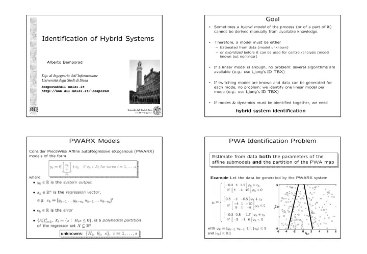
Goal Goal

• Sometimes a hybrid model of the process (or of a part of it)

cannot be derived manually from available knowledge.

• Therefore, a model must be either

– Estimated from data (model unknown) – or hybridized before it can be used for control/analysis (model known but nonlinear)

• If a linear model is enough, no problem: several algorithms are

available (e.g.: use Ljung’s ID TBX)

• If switching modes are known and data can be generated for

each mode, no problem: we identify one linear model per mode (e.g.: use Ljung’s ID TBX)

• If modes & dynamics must be identified together, we need

hybrid system identification

PWARX PWARX Models Models

Consider PieceWise Affine autoRegressive eXogenous (PWARX) models of the form where: unknowns:

PWA PWA Identification Problem Identification Problem

Estimate from data both the parameters of the affine submodels and the partition of the PWA map

Example Let the data be generated by the PWARX system

PWA PWA Identification Problem Identification Problem

• A. Known Guardlines (partition Hj known, θj unknown):
• rdinary least-squares problem (or linear/quadratic program if

linear bounds over θj are given) EASY PROBLEM

• B. Unknown Guardlines (partition Hj and θj unknown):

generally non-convex, local minima HARD PROBLEM!

• Polynomial factorization (algebraic approach)
• Hyperplane clustering in data space

Approaches to Approaches to PWA PWA Identification Identification

• Mixed-integer linear or quadratic programming
• Bounded error & partition of infeasible set of

inequalities

• K-means clustering in a feature space
• A. Bemporad, A. Garulli, S. Paoletti and A. Vicino, “A Greedy Approach

to Identification of Piecewise Affine Models”, HSCC’03

• G. Ferrari-Trecate, M. Muselli, D. Liberati, and M. Morari, “A clustering

technique for the identification of piecewise affine systems”, Automatica, 2003

• J. Roll, A. Bemporad and L. Ljung, “Identification of hybrid systems via

mixed-integer programming”, Automatica, to appear. (R. Vidal, S. Soatto,

• S. Sastry, 2003)

(E. Münz, V. Krebs, IFAC 2002)

• Other approaches:

Mixed Mixed-

• Integer Approach

Integer Approach Mixed Mixed-

• Integer Approach

Integer Approach

Hinging Hyperplane hybrid models + +

Example:

(Breiman, 1993)

Mixed Mixed-

• Integer Approach

Integer Approach

• ne-step ahead

predicted output (t=0, 1, ..., N-1)

• ptimization problem:
• Could be solved using numerical methods such as the

Gauss-Newton method. (Breiman, 1993)

• Problem: Local minima.
• We want to find a method that finds the global

minimum

Mixed Mixed-

• Integer Approach

Integer Approach

• A general Mixed-Integer Quadratic Program (MIQP)

can be written as (if Q=0 the problem is an MILP) 1. If we set , we get the cost function becomes quadratic in (θi,zi(t)):

Mixed Mixed-

• Integer Approach

Integer Approach

• 2. Introduce binary variables
• 3. Get linear mixed-integer constraints:

(if-then-else condition)

• ε is a small positive scalar (e.g., the machine precision),
• M and m are upper and lower bounds on (from bounds on θi)

The identification problem is an MIQP !

Mixed Mixed-

• Integer Approach

Integer Approach

Example: Identify the following system MILP: 66 variables (of which 20 integers) and 168 constraints. Problem solved using Cplex 6.5 (1014 LP solved in 0.68 s)

Mixed Mixed-

• Integer Approach

Integer Approach

System identified using noiseless data Using data with Var(e(t))=0.1 Fitting an ARX model to same data (Var(e(t))=0.1)

Problem: Worst-case complexity is exponential in the number of hinge functions and in the number of data.

Mixed Mixed-

• Integer Approach

Integer Approach

Wiener models:

• Linear system G(z) followed by a one dimensional static

nonlinearity f.

• Assumptions: f is piecewise affine, continuous, invertible ⇒

the system is piecewise affine.

x y u

• The identification problem can be again solved via MIQP or

MILP

• Complexity is polynomial in worst-case in the number of data

and number of max function

• Still the complexity depends heavily on the number of data

Result:

Mixed Mixed-

• Integer Approach

Integer Approach

• Global optimal solution can be obtained
• A 1-norm objective function gives an MILP problem

a 2-norm objective function gives an MIQP problem

• Worst-case performance is exponential in the number

functions and quite bad in the number of data! Comments: Need to find methods that are suboptimal but computationally more efficient !

Bounded Bounded-

• Error Approach

Error Approach

Bounded Error Condition Bounded Error Condition

Consider again a PWARX model of the form Bounded-error: select a bound δ>0 and require that the identified model satisfies the condition Problem Given N datapoints (yk,xk), k=1, ..., N, estimate the min integer s, a partition , and params θ1, ... ,θs such that the corresponding PWA model satisfies the bounded error condition Role of δ: trade off between quality of fit and model complexity

MIN MIN PFS PFS Problem Problem

Given δ>0 and the (possibly infeasible) system of N linear complementary inequalities find a partition of this system of inequalities into a minimum number s of feasible subsystems of inequalities Problem restated as a MIN PFS problem:

(MINimum Partition into Feasible Subsystems)

• The partition of the complementary ineqs provides data

classification (=clusters)

• Each subsystem of ineqs defines the set of linear models θi

that are compatible with the data in cluster #i

• MIN PFS is an NP-hard problem

A Greedy Algorithm for MIN A Greedy Algorithm for MIN PFS PFS

• A. Starting from an infeasible set of inequalities, choose a

parameter θ that satisfies the largest number of ineqs

(Amaldi & Mattavelli, Disc. Appl. Math., 2002)

and classify those satisfied ineqs as the first cluster (MAXimum Feasible Subsystem, MAX FS)

• B. Iteratively repeat the MAX FS problem on the remaining ineqs
• The MAX FS problem is still NP-hard
• Amaldi & Mattavelli propose to tackle it using a randomized

and thermal relaxation method

PWA PWA Identification Algorithm Identification Algorithm

• 1. Initialize: exploit a greedy strategy for partitioning

an infeasible system of linear inequalities into a minimum number of feasible subsystems

• 2. Refine the estimates: alternate between datapoint

reassignment and parameter update

• 3. Reduce the number of submodels:
• a. join clusters whose model θi is similar, or
• b. remove clusters that contain too few points
• 3. Estimate the partition: compute a separating

hyperplane for each pair of clusters of regression vectors (alternative: use multi-category classification techniques)

Step #1: Greedy Algorithm for MIN Step #1: Greedy Algorithm for MIN-

• PFS

PFS

Comments on the greedy algorithm

• The greedy strategy is not guaranteed to yield a minimum

number of partitions (it solves MIN PFS only suboptimally)

• Randomness involved for tackling the MAX FS problem
• The cardinality and the composition of the clusters may

depend on the order in which the feasible subsystems are extracted

• Some datapoints might be consistent with more than one

submodel

The greedy strategy can only be used for initialization

• f the clusters. Then we need a procedure for the

refinement of the estimates

Example (cont’d) Example (cont’d)

Consider again the PWARX system

greedy algorithm

initial classification (6 clusters → quite rough)

Step #2: Refinement Procedure Step #2: Refinement Procedure

(linear programming)

Step #2: Comments Step #2: Comments

Comments about the iterative procedure

• Why the projection estimate?
• Why the distinction among infeasible, undecidable, and

feasible datapoints?

No feasible datapoint at refinement t becomes infeasible at refinement t+1

• Infeasible datapoints are not consistent with any submodel, and may be
• utliers ⇒ neglecting them helps improving the quality of the fit
• Undecidable datapoints are consistent with more than one submodel

⇒ neglecting them helps to reduce misclassifications

Step #3: Reduce Number of Step #3: Reduce Number of Submodels Submodels

• Similarity of the parameter vectors
• Cardinality of the clusters

Thresholds α and β should be suitably chosen in order to reduce the number of submodels still preserving a good fit of the data

Example (cont’d) Example (cont’d)

Consider again the PWARX system

Classification of the regression vectors after the refinement (3 clusters) Number of undecidable datapoints vs number of refinements

Step #4: Estimation of the Partition Step #4: Estimation of the Partition

Estimation of the partition of the regressor set

• This step can be performed by computing a separating

hyperplane for each pair of final clusters Fi of regression vectors

• If two clusters Fi and Fj are not linearly separable, look for a

hyperplane that minimizes the number of misclassified points (generalized separating hyperplane)

• Linear Support Vector Machines (SVMs) can be used to

compute the optimal generalized separating hyperplane of two clusters Alternative: use multi-category classification techniques (computationally more demanding, but better results)

(Bennet and Mangasarian, 1992)

Step #4: Estimation of the Partition Step #4: Estimation of the Partition

• Given two clusters Fi and Fj, a separating hyperplane

'

x a+b=0 is such that Generalized separating hyperplane and MAX FS

• A solution of the MAX FS problem of the above system of

ineqs is a hyperplane that minimizes the number of misclassified points

• The misclassified points, if any, are removed from Fi and/or Fj
• Then, compute the optimal separating hyperplane of Fi and Fj

via quadratic programming

'

x a+b=-1

'

x a+b=1

Example (cont’d) Example (cont’d)

Consider again the PWARX system Final classification of the regression vectors, and true (dashed lines) and estimated (solid lines) partition of the regressor set

Example 2: Nonlinear Example 2: Nonlinear Fnc Fnc Approx. Approx.

We want to hybridize the nonlinear function

N=1000 datapoints, δ=0.05, α=10%, β=1%

s=6 submodels (CPU time: 5.7 s, PIII 1GHz)

Feature Space Clustering Approach Feature Space Clustering Approach

(thanks to G.Ferrari-Trecate for providing this material)

Assumptions ( Assumptions (PWARX PWARX Model) Model)

• Model orders , fixed

na n b

The switching law is assumed unknown: Both the submodels and the shape of the regions must be estimated from the dataset

• The number of submodels is known

s

Dataset: S = {(x(k), y(k)), k = 1, . . ., N}

Hybrid Identification Algorithm Hybrid Identification Algorithm

Regression Pattern Recognition Clustering

f:R

n7→

R f:R

n7→

{0 1 ... p} Learning from a finite dataset

Reconstruction

• f continuous

behaviors (dynamics) Reconstruction

• f discrete

behaviors (switching)

Hybrid Identification

Toy Example Toy Example

• datapoints

N = 50

ïk ø N(0, 0.01) X3 X2 X1 y(k) = u(k à 1) + 2 + ï(k) à u(k à 1) + ï(k) u(k à 1) + 2 + ï(k)    u(k à1) ∈ X1 u(k à1) ∈ X2 u(k à1) ∈ X3

if if if

• Dataset

The first and the third submodel have the same coefficients (but they are defined on different regions) C2 C1

Step #1: Build Local Datasets Step #1: Build Local Datasets

The PWARX model is locally linear: Small sets of datapoints that are close to each other are likely to belong to the same submodel For each datapoint x(j ), y(j) ( ) build a set Cj collecting x(j), y(j) ( ) and the first neighboring points ( )

c>na +nb +1

c à 1

There is a one-to-one map between each Sets collecting points belonging to a single subsystem: Pure sets (e.g. )

C1

Sets collecting points belonging to different subsystems: Mixed sets (e.g. )

C2 Cj

x(j), y(j) ( ) and the datapoint set

x(1)

Step #2: Identification of Local Models Step #2: Identification of Local Models

For each local dataset identify an affine model through least squares (vector of coefficients: )

C 2

C 1 Cj

• Mixed sets should give isolated vectors of coefficients ò

LS,j

"High" S/N ratio and few mixed sets ⇒ Clusters of vectors + few outliers Outlier Clusters

òLS,j òLS,j

• Pure sets collecting datapoints belonging to the same submodel should

produce similar òLS,j

C 3

The Feature Vectors The Feature Vectors

Problem: The same vector of coefficients can characterize submodels defined on different regions (Ferrari-Trecate et. al, HSCC 2001) Consider the feature vectors

mj = c

1 P (x,y)∈Cj x

øj = òLS,j m

j

ô õ The vector takes into account the spatial localization of the -th local model

øj j

Outlier 3 Clusters Exploit such measures in a "K-means like" algorithm that divides the feature vectors in subsets ,

Step #3: Clustering the feature vectors Step #3: Clustering the feature vectors

Outlier 3 Clusters Next problem: find the clusters in the feature space The accuracy must not be spoiled by the outliers Introduce measures of the confidence one should have about the fact that is based

• n a mixed local dataset

øj D i i=1,...,s

The clustering algorithm proposed in (Ferrari-Trecate et. al, HSCC 2001) guarantees convergence to a (possibly suboptimal) set of clusters in a finite number of iterations

Clustering Step (Toy Example) Clustering Step (Toy Example) D 1 D 2 D 3

Outlier Unclassified feature vectors Classified feature vectors

Step #4: Classification of the Step #4: Classification of the Datapoints Datapoints

Build the sets of classified datapoints according to the rule

Fi i=1,...,s

if , then

øj ∈D

i

x(j),y(j) ( ) ∈ Fi F 1 F 2 F 3

Step #5: Identification of the Step #5: Identification of the Submodels Submodels

Use the data in each set for estimating both the affine submodels and the regions

F i

F 1 F 2 F 3

Submodel coefficients: Weighted Least Squares exploiting the confidence measures

• Linear Support Vector Machines
• Multicategory Robust Linear Programming

(Bennet & Mangasarian, 1992) (Vapnik, 1998)

• solved via linear/quadratic programming

Shape of the polyhedral regions:

Toy Problem: Identification Results Toy Problem: Identification Results

Computational time: 1.26 s. (on a Pentium 600 Mhz running Matlab 5.3) True model Identified model

y(k)= u(kà1) +2 +ï(k) àu(kà1)+ï(k) u(kà1) +2 +ï(k)    u(kà1) ∈[à4,à1) u(kà1)∈[à1,2] u(kà1)∈[2,4] y(k)= u(kà1) +1.99+ï(k) à1.05u(kà1) +0.01+ï(k) 1.02u(kà1)+1.92+ï(k)    u (kà1 )∈[à4 ,à0 .8 ] u (kà1 )∈[à0 .8 ,1 .8 ] u (kà1 )∈[1 .8,4]

Example: Industrial Transformer Example: Industrial Transformer

Industrial transformers used in a protection system:

• The measurement of is difficult and costly
• The measurement of is easy

i1(t) i2(t)

Goal: Estimate from

i1(t) i2(t)

Problems:

• Hysteresis and saturations occur for currents of high intensity
• Derive a model for simulation
• Sampling time: 5.0000e-005 s.

(S. Bittanti et al., 2001)

Identified PWARX model Identified PWARX model

i1(k) =aj,1i2(kà1) +aj,24i2(kà1) [i2(kà1) ∆i2(kà1)] ∈X

j

j =1,...,5 Identified submodels and classified datapoints (440 measurements) PWARX model (five regions) Computational time: 15.76 s. (Pentium 600 Mhz, Matlab 5.3) Local datasets of 50 points

Cj

Validation Results Validation Results

Predicted (--) and true primary current

• There are nonlinear (ad hoc) simulators for industrial transformers

(S. Bittanti et al., 2001)

Advantage of PWARX models: Simple enough for on-line implementation

Conclusions Conclusions

• Main goal of hybrid systems identification:

– Develop simple switching models from data (or from more complex models) to be used for control/analysis purposes

• Hybrid system identification is a hard problem
• Theory is still in its infancy
• Some algorithms are already available
• Applications:

– Biomedical (Analysis of the EEG ⇒ Brain-Computer interface; Dialysis: early assessment of the therapy duration) – Ecological (trophic, oxygen and nutrient dynamics in aquatic systems) – ... (many others !)