I i M i M i 5 6 Handling non-Global Alignments Original profile - - PDF document

SLIDE 1

CSCE 471/871 Lecture 4: Profile Hidden Markov Models

Stephen D. Scott

1

Introduction

• Designed to model (profile) a multiple alignment of a protein family

(e.g. p. 102)

• Gives a probabilistic model of the proteins in the family
• Useful for searching databases for more homologues and for aligning

strings to the family

2

Outline

• Organization of a profile HMM

– Ungapped regions – Insert and delete states

• Building a model
• Searching with HMMs

3

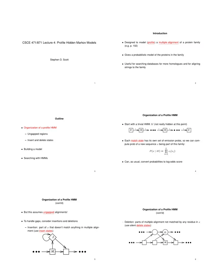
Organization of a Profile HMM

• Start with a trivial HMM M (not really hidden at this point)

B

1

M1

1

M E

i

1 1 1

• Each match state has its own set of emission probs, so we can com-

pute prob of a new sequence x being part of this family: P(x | M) =

L Y i=1

ei(xi)

• Can, as usual, convert probabilities to log-odds score

4

Organization of a Profile HMM (cont’d)

• But this assumes ungapped alignments!
• To handle gaps, consider insertions and deletions

– Insertion: part of x that doesn’t match anything in multiple align- ment (use insert states)

Mi

i

I

5

Organization of a Profile HMM (cont’d)

• Deletion: parts of multiple alignment not matched by any residue in x

(use silent delete states) Mi D

i

6

SLIDE 2

General Profile HMM Structure

E B

7

Handling non-Global Alignments

• Original profile HMMs model entire sequence
• Add flanking model states (or free insertion modules) to generate non-

local residues

B E

8

Outline

• Organization of a profile HMM
• Building a model

– Structure – Estimating probabilities

• Searching with HMMs

9

Building a Model

• Given a multiple alignment, how to build an HMM?

– General structure defined, but how many match states?

... V - - - - N V D E V ... ... V E A - - D V A G H ... ... V K G - - - - - - D ... ... V Y S - - T Y E T S ... ... F N A - - N I P K H ... ... I A G A D N G A G V ... ... V G A - - H A G E Y ...

10

Building a Model (cont’d)

• Given a multiple alignment, how to build an HMM?

– General structure defined, but how many match states? – Heuristic: if more than half of characters in a column are non-gaps, include a match state for that column

... V - - - - N V D E V ... ... V E A - - D V A G H ... ... V K G - - - - - - D ... ... V Y S - - T Y E T S ... ... F N A - - N I P K H ... ... I A G A D N G A G V ... ... V G A - - H A G E Y ...

11

Building a Model (cont’d)

• Now, find parameters
• Multiple alignment + HMM structure ! state sequence

match state Gap in match column -> delete state Non-gap in insert column -> insert state Gap in insert column -> ignore Durbin Fig 5.4, p. 109 Non-gap in match column -> ... V - - - - N V D E V ... ... V E A - - D V A G H ... ... V K G - - - - - - D ... ... V Y S - - T Y E T S ... ... F N A - - N I P K H ... ... I A G A D N G A G V ... ... V G A - - H A G E Y ... M1 D3 I3

12

SLIDE 3

Building a Model (cont’d)

• Count number of transitions and emissions and compute:

akl = Akl

P l0 Akl0

ek(b) = Ek(b)

P b0 Ek(b0)

• Still need to beware of some counts = 0

13

Weighted Pseudocounts

• Let cja = observed count of residue a in position j of

multiple alignment eMj(a) = cja + Aqa

P a0 cja0 + A

• qa = background probability of a, A = weight placed on

pseudocounts (sometimes use A ⇡ 20)

• Background probabilities also called a prior distribution

14

Dirichlet Mixtures

• Can be thought of as a mixture of pseudocounts
• The mixture has different components, each representing a different

context of a protein sequence – E.g. in parts of a sequence folded near protein’s surface, more weight (higher qa) can be given to hydrophilic residues – But in other regions, may want to give more weight to hydrophobic residues

• Will find a different mixture for each position of the alignment based on

the distribution of residues in that column

15

Dirichlet Mixtures (cont’d)

• Each component k consists of a vector of pseudocounts ~

↵k (so ↵k

a

corresponds to Aqa) and a mixture coefficient (mk, for now) that is the probability that component k is selected

• Pseudocount model k is the “correct” one with probability mk
• We’ll set the mixture coefficients for each column based on which vec-

tors best fit the residues in that column – E.g. first column of alignment on slide 10 is dominated by V, so any vector ~ ↵k that favors V will get a higher mk

16

Dirichlet Mixtures (cont’d)

• Let ~

cj be vector of counts in column j eMj(a) =

X k

P

⇣

k | ~ cj

⌘

cja + ↵k

a P a0 ⇣

cja0 + ↵k

a0 ⌘

• P

⇣

k | ~ cj

⌘

are the posterior mixture coefficients, which are easily com- puted [Sj¨

• lander et al. 1996], yielding:

eMj(a) = Xa

P a0 Xa0 ,

where Xa =

X k

mk0 exp

⇣

ln B

⇣

~ ↵k + ~ cj

⌘

ln B

⇣

~ ↵k⌘⌘ cja + ~ ↵k

a P a0 ⇣

cja0 + ↵k

a0 ⌘ ,

ln B(~ x) =

X i

ln Γ(xi) ln Γ

@X i

xi

1 A

17

Dirichlet Mixtures (cont’d)

• Γ is gamma function, and ln Γ is computed via lgamma and related

functions in C

• mk0 is prior probability of component k (= q in Sj¨
• lander Table 1):

. . .

18

SLIDE 4

Outline

• Organization of a profile HMM
• Building a model
• Searching with HMMs

19

Searching for Homologues

• Score a candidate match x by using log-odds:

– P(x, ⇡⇤ | M) is probability that x came from model M via most likely path ⇡⇤ ) Find using Viterbi – Pr(x | M) is probability that x came from model M summed over all possible paths ) Find using forward algorithm – score(x) = log(P(x | M)/P(x | )) ⇤ is a “null model”, which is often the distribution of amino acids in the training set or AA distribution over each individual column ⇤ If x matches M much better than , then score is large and positive

20

Viterbi Equations

• V M

j

(i) = log-odds score of best path matching x1...i to the model, where xi emitted by state Mj (similarly define V I

j (i) and V D j (i))

• Rename B as M0, V M

0 (0) = 0, rename E as ML+1 (V M L+1 = final)

V M

j

(i) = log

eMj(xi)

qxi

!

+ max

8 > > < > > :

V M

j1(i 1) + log aMj1Mj

V I

j1(i 1) + log aIj1Mj

V D

j1(i 1) + log aDj1Mj

V I

j (i) = log eIj(xi)

qxi

!

+ max

8 > > < > > :

V M

j

(i 1) + log aMjIj V I

j (i 1) + log aIjIj

V D

j (i 1) + log aDjIj

V D

j (i) = max 8 > > < > > :

V M

j1(i) + log aMj1Dj

V I

j1(i) + log aIj1Dj

V D

j1(i) + log aDj1Dj

• Similar to Chapter 2’s gapped alignment, but with position-specific

scoring scheme

21

Forward Equations F M

j (i) = log eMj(xi)

qxi

!

+ log

h

aMj1Mj exp

⇣

F M

j1(i 1) ⌘

+ aIj1Mj exp

⇣

F I

j1(i 1) ⌘

+ aDj1Mj exp

⇣

F D

j1(i 1) ⌘i

F I

j (i) = log eIj(xi)

qxi

!

+ log

h

aMjIj exp

⇣

F M

j (i 1) ⌘

+ aIjIj exp

⇣

F I

j (i 1) ⌘

+ aDjIj exp

⇣

F D

j (i 1) ⌘i

F D

j (i) = log h

aMj1Dj exp

⇣

F M

j1(i) ⌘

+ aIj1Dj exp

⇣

F I

j1(i) ⌘

+aDj1Dj exp

⇣

F D

j1(i) ⌘i

• exp(·) needed to use sums and logs (can still be fast; see p. 78)

22

Aligning a Sequence with a Model (Multiple Alignment)

• Given a string x, use Viterbi to find most likely path ⇡⇤ and use the

state sequence as the alignment

• More detail in Durbin, Section 6.5

– Also discusses building an initial multiple alignment and HMM si- multaneously via Baum-Welch

23

Topic summary due in 1 week!

24