[PPT] - I Can See Clearer Now The Blur is Gone Per Christian Hansen PowerPoint Presentation

SLIDE 1

GAMM 2008

1

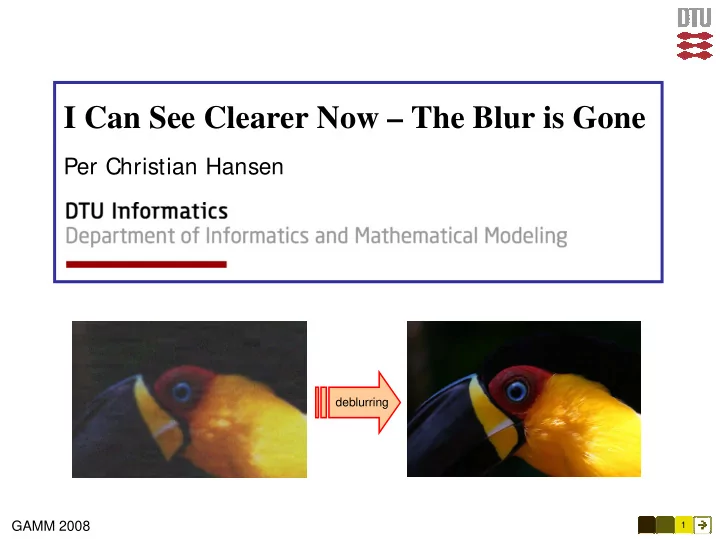
I Can See Clearer Now – The Blur is Gone

Per Christian Hansen

deblurring

SLIDE 2

GAMM 2008

2

The Speaker

Per Christian Hansen

Professor of Scientific Computing at DTU
MSc EE 1982 – PhD Num. Anal. 1985 – Dr Techn 1996
Key interests: large-scale computing & inverse problems

Author of two books on inverse problems:

SLIDE 3

GAMM 2008

3

Sources of Blurred Images

SLIDE 4

GAMM 2008

4

Some Types of Blur and Distortion

From the camera:

the lens is out of focus,
imperfections in the lens, and
noise in the CCD and the analog/digital converter.

From the environments:

motion of the object (or camera),
fluctuations in the light’s path (turbulence), and
false light, cosmic radiation (in astronomical images).

Given a mathematical/statistical model of the blur and distortion, we can deblur the image and compute a sharper reconstruction.

SLIDE 5

GAMM 2008

5

Some Applications of Deblurring

Astronomical imaging Biometrics and surveillance Image deblurring Fingerprint restoration Image in-painting

SLIDE 6

GAMM 2008

6

Mathematics of Image Deblurring

blurring deblurring

Io (moon of Jupiter) You cannot depend on your eyes when your imagination is out of focus

– Mark Twain

SLIDE 7

GAMM 2008

7

Same Problem: Inverse Acoustics

SLIDE 8

GAMM 2008

8

Same Problem: Inverse Geomagnetism

SLIDE 9

GAMM 2008

9

Same Problem: Seismic Tomography

Seismographs Surface Colors represent slowness (recip.

f sound speed).

Incoming seismic waves Reconstruction

SLIDE 10

GAMM 2008

10

The Point Spread Function

SLIDE 11

GAMM 2008

11

Discretization: Equations → Numbers

SLIDE 12

GAMM 2008

12

Discretization: Equations → Numbers

Examples of point spread functions

SLIDE 13

GAMM 2008

13

The Difficult Task of Image Deblurring

SLIDE 14

GAMM 2008

14

Inverse Problems

Inverse problems are examples of ill-posed problems:

the solution may not exist,
the solution may not be unique, or
the solution may not depend continuously on data.

Example: the world’s simplest ill-posed problem: x1 + x2 = 1. The linear systems of equations associated with discretizations of linear inverse problems are effectively underdetermined – even if the system A x = b is square or overdetermined.

SLIDE 15

GAMM 2008

15

Structured Matrices

The matrix A in image deblurring problems is often structured. Typically, it is BTTB = block Toeplitz with Toeplitz blocks.

SLIDE 16

GAMM 2008

16

Professor Toeplitz and his Matrix

Otto Toeplitz, 1881 – 1940. Worked on linear and quadratic forms. Given a stationary time series x1, x2, x3, x4, ... the autocorrelation matrix, with elements cij = ai-j = cov(xi , xj ) , is a Toeplitz matrix.

SLIDE 17

GAMM 2008

17

Utilization of Matrix Structure

Ordinary matrix-vector multiplication flop count. Toeplitz matrix-vector multiplication flop count.

SLIDE 18

GAMM 2008

18

The FFT Algorithm

The ”fathers” – published 1965. The definition The algorithm

function y = fft(x) % FFT algorithm, n = power-of-2 n = length(x);

mega = exp(-2*pi*i/n);

if n > 2 % Recursive divide and conquer. k = (0:n/2-1)'; w = omega.^k; u = fft(x(1:2:n-1)); v = w.*fft(x(2:2:n)); y = [u+v; u-v]; else % The Fourier matrix. j = 0:n-1; k = j'; F = omega.^(k*j); y = F*x; end

The principle – O(n log(n) ) complexity

SLIDE 19

GAMM 2008

19

FFT-Based Methods

We can immediately reconstruct the image via FFT computations:

Periodic boundary conditions:

F = ifft2( fft2(G) ./ fft2(P) );

with Wiener filtering

S = fft2(P); % Eigenvalues. F = ifft2( (S./(S.^2 + lambda) .* fft2(G) )

Reflexive boundary conditions (and symmetric PSF):

S = dct2(P) ./ dct2(e1); % Eigenvalues. F = idct2( dct2(G) ./ S )

with filtering

Q = dct2(P) ./ dct2(e1); % Eigenvalues. F = idct2( (S./(S.^2 + lambda) .* dct2(G) )

For details, see the book

SLIDE 20

GAMM 2008

20

Regularizing Iterations

SLIDE 21

GAMM 2008

21

Krylov Signal Subspaces

Smiley Crater, Mars

SLIDE 22

GAMM 2008

22

Top 10 Algorithms

J.J. Dongarra, F. Sullivan et al., The Top 10 Algorithms, IEEE Computing in Science and Engineering, 2 (2000), pp. 22-79. 1946: The Monte Carlo method (Metropolis Algorithm). 1947: The Simplex Method for Linear Programming. 1950: Krylov Subspace Methods (CG, CGLS, Arnoldi, etc.). 1951: Decomposition Approach to matrix computations. 1957: The Fortran Optimizing Compiler. 1961: The QR Algorithm for computing eigenvalues and –vectors. 1962: The Quicksort Algorithm. 1965: The Fast Fourier Transform algorithm. 1977: The Integer Relation Detection Algorithm. 1987: The Fast Multipole Algorithm for N-body simulations. 1946: The Monte Carlo method (Metropolis Algorithm). 1947: The Simplex Method for Linear Programming. 1950: Krylov Subspace Methods (CG, CGLS, Arnoldi, etc.). 1951: Decomposition Approach to matrix computations. 1957: The Fortran Optimizing Compiler. 1961: The QR Algorithm for computing eigenvalues and –vectors. 1962: The Quicksort Algorithm. 1965: The Fast Fourier Transform algorithm. 1977: The Integer Relation Detection Algorithm. 1987: The Fast Multipole Algorithm for N-body simulations. Key algorithms in image deblurring.

SLIDE 23

GAMM 2008

23

Semi-Convergence of CGLS

SLIDE 24

GAMM 2008

24

Progress of the Iterations

Initially, the image gets sharper – then ”freckles” start to appear.

DCT spectrum spatial domain

The ”freckles” are band-pass filtered noise.

SLIDE 25

GAMM 2008

25

Away From 2-Norms

Io (moon of Saturn) q = 1.1 q = 2

SLIDE 26

GAMM 2008

26

Total Variation In-Painting

C S I : C o m p u t a t i o n a l S c i e n c e i n I m a g i n g

Matlab and C software (working title: TV box) is almost finished.

SLIDE 27

GAMM 2008

27

3D Tomography in Crystallography

Data:

X-ray diffraction

Reconstruction:

rientation distribution function

Smoothing norm:

|| ∇2f ||2 Solution shows the distribution of

rientations in an imperfect crystal.

Joint work with Metals in 4D, Risø DTU