HW/SW Codesign Data Flow Software Implementation I ECE 522 Mapping - - PowerPoint PPT Presentation

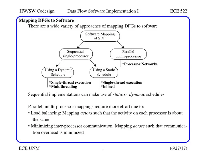
HW/SW Codesign Data Flow Software Implementation I ECE 522 ECE UNM 1 (6/27/17) Mapping DFGs to Software There are a wide variety of approaches of mapping DFGs to software Sequential implementations can make use of static or dynamic schedules Parallel, multi-processor mappings require more effort due to:

• Load balancing: Mapping actors such that the activity on each processor is about

the same

• Minimizing inter-processor communication: Mapping actors such that communica-

tion overhead is minimized

Software Mapping

• f SDF

Sequential single-processor Parallel multi-processor *Processor Networks Using a Static Schedule *Single-thread execution *Inlined Using a Dynamic Schedule *Single-thread execution *Multithreading

HW/SW Codesign Data Flow Software Implementation I ECE 522 ECE UNM 2 (6/27/17) Mapping DFGs to Software We focus first on single-processor systems, and in particular, on finding efficient ver- sions of sequential schedules As noted on the previous slide, there are two options for implementing the schedule:

• Dynamic schedule

Here, software decides the order in which actors execute at runtime by testing firing rules to determine which actor can run Dynamic scheduling can be done in a single-threaded or multi-threaded execu- tion environment

• Static schedule

In this case, the firing order is determined at design time and fixed in the imple- mentation The fixed order allows for a design time optimization in which the firing of mul- tiple actors can be treated as a single firing This in turn allows for ’inlined’ implementations

HW/SW Codesign Data Flow Software Implementation I ECE 522 ECE UNM 3 (6/27/17) DFG Elements Before discussing these, let’s first look at C implementations of actors and queues FIFO Queues: Although DFGs theoretically have infinite length queues, in practice, queues are lim- ited in size We discussed earlier that constructing a PASS allows the maximum queue size to be determined by analyzing actor firing sequences A typical software interface of a FIFO queue has two parameters and three methods

• The # of elements N that can be stored in the queue and the data type of the ele-

ments

• Methods that put elements into the queue, get elements from the queue, and query

the current size of the queue void Q.put(element &) void & Q.get() N unsigned Q.getsize()

HW/SW Codesign Data Flow Software Implementation I ECE 522 ECE UNM 4 (6/27/17) DFG Elements Queues are well defined (standardized) data structures A circular queue consists of an array, a write-pointer and a read-pointer They use modulo addressing, e.g., the Ith element is at position (Rptr + I) mod Q.getsize() Example fifo data structure definition in C: #define MAXFIFO 1024 typedef struct fifo { int data[MAXFIFO]; // array unsigned wptr; // write pointer unsigned rptr; // read pointer } fifo_t;

Queue Wprt Rprt Queue Wprt Rprt 5 Queue Wprt Rprt 5 6 Init After ’put(5)’ After ’put(6)’ Queue Wprt Rprt 5 6 ’put(2)’ -- NO! Queue is Full

HW/SW Codesign Data Flow Software Implementation I ECE 522 ECE UNM 5 (6/27/17) DFG Elements void init_fifo(fifo_t *F); // These functions defined void put_fifo(fifo_t *F, int d); // in text int get_fifo(fifo_t *F); unsigned fifo_size(fifo_t *F); int main() { fifo_t F1; init_fifo(&F1); // resets wptr, rptr put_fifo(&F1, 5); put_fifo(&F1, 6); printf("%d %d\n", fifo_size(&F1), get_fifo(&F1)); printf("%d\n", fifo_size(&F1)); // prints 1 } Note that the queue size is fixed here at compile time Alternatively, queue size can be changed dynamically at runtime using malloc()

HW/SW Codesign Data Flow Software Implementation I ECE 522 ECE UNM 6 (6/27/17) DFG Elements Actors: An actor can be represented as a C function, with an interface to the FIFOs The actor function incorporates a finite state machine (FSM), which checks the firing rules to determine whether to execute the actor code The local controller (FSM) of an actor has two states wait state: start state which checks the firing rules immediately after being invoked by a scheduler work state: wait transitions to work when firing rules are satisfied The actor then reads tokens, performs calculation and writes output tokens

HW/SW Codesign Data Flow Software Implementation I ECE 522 ECE UNM 7 (6/27/17) Example C Implementation of DFG An example which supports up to 8 inputs and outputs per actor: #define MAXIO 8 typedef struct actorio { fifo_t *in[MAXIO], *out[MAXIO]; } actorio_t; An example actor implementation: void fft2(actorio_t *g) { int a, b; if( fifo_size(g->in[0]) >= 2 ) // Firing rule check { a = get_fifo(g->in[0]); b = get_fifo(g->in[0]); put_fifo(g->out[0], a+b); put_fifo(g->out[0], a-b); } }

HW/SW Codesign Data Flow Software Implementation I ECE 522 ECE UNM 8 (6/27/17) Mapping DFGs to Single Processors: Dynamic Schedule In a dynamic system schedule, the firing rules of the actors are tested at runtime In a single-thread dynamic schedule, we implement the system scheduler as a func- tion that instantiates ALL actors and queues The scheduler typically calls the actors in a round-robin fashion void main() { fifo_t q1, q2; actorio_t fft2_io = {{&q1}, {&q2}}; ... init_fifo(&q1); init_fifo(&q2); while (1) { fft2_actor(&fft2_io); // .. call other actors } }

HW/SW Codesign Data Flow Software Implementation I ECE 522 ECE UNM 9 (6/27/17) Mapping DFGs to Single Processors: Dynamic Schedule Note that it is impossible to call the actors in the wrong order This is true b/c each of them checks a firing rule that prevents them from run- ning when there is no data available An interesting question is ’is there a call order of the actors that is best?’ The schedule on the right shows that snk in (a) is called as often as src However, snk will only fire on even numbered invocations (b) shows a problem that is not handled by static schedulers Round-robin scheduling in this case will eventually lead to queue overflow

HW/SW Codesign Data Flow Software Implementation I ECE 522 ECE UNM 10 (6/27/17) Mapping DFGs to Single Processors: Dynamic Schedule The underlying problem with (b) is that the implemented firing rate differs from the firing rate for a PASS, which is given as (src, snk, snk) There are two solutions to this issue:

• Adjust the system schedule to match the PASS

void main() { .. while (1) { src_actor(&src_io); snk_actor(&snk_io); snk_actor(&snk_io); } } Unfortunately, this solution defeats one of the goals of a dynamic scheduler, i.e., that it automatically converges to the PASS firing rate

HW/SW Codesign Data Flow Software Implementation I ECE 522 ECE UNM 11 (6/27/17) Mapping DFGs to Single Processors: Dynamic Schedule

• A better solution is to add a while loop to the snk actor code to allow it to continue

execution while there are tokens in the queue void snk_actor(actorio_t *g) { int r1, r2; while ((fifo_size(g->in[0]) > 0)) { r1 = get_fifo(g->in[0]); ... // do processing } }

HW/SW Codesign Data Flow Software Implementation I ECE 522 ECE UNM 12 (6/27/17) Mapping DFGs to Single Processors: Example Dynamic Schedule Let’s implement the 4-point Fast Fourier Transform (FFT) shown above using a dynamic schedule The array t stores 4 (time domain) samples The array f will be used to store the frequency domain representation of t The FFT utilizes butterfly operations to implement the FFT, as defined on the right side in the figure The twiddle factor W(k, N) is a complex number defined as e-j2πk/N, with W(0, 4) = 1 and W(1, 4) = -j

HW/SW Codesign Data Flow Software Implementation I ECE 522 ECE UNM 13 (6/27/17) Mapping DFGs to Single Processors: Example Dynamic Schedule The DFG for (a) is given as follows

• reorder: Reads 4 tokens and shuffles them to match the flow diagram

The t[0] and t[2] are processed by the top butterfly and t[1] and t[3] are pro- cessed by the bottom butterfly

• fft2: Calculates the butterflies for the left half of the flow diagram
• fft4mag calculates the butterflies for the right half and produces the magnitude com-

ponent of the frequency domain representation

HW/SW Codesign Data Flow Software Implementation I ECE 522 ECE UNM 14 (6/27/17) Mapping DFGs to Single Processors: Example Dynamic Schedule The implementation first requires a valid schedule to be computed The firing rate is easily determined to be [qreorder, qfft2, qfft4mag] = [1, 2, 1] void reorder(actorio_t *g) { int v0, v1, v2, v3; while ( fifo_size(g->in[0]) >= 4 ) { v0 = get_fifo(g->in[0]); v1 = get_fifo(g->in[0]); v2 = get_fifo(g->in[0]); v3 = get_fifo(g->in[0]); put_fifo(g->out[0], v0); put_fifo(g->out[0], v2); put_fifo(g->out[0], v1); put_fifo(g->out[0], v3); } }

HW/SW Codesign Data Flow Software Implementation I ECE 522 ECE UNM 15 (6/27/17) Mapping DFGs to Single Processors: Example Dynamic Schedule void fft2(actorio_t *g) { int a, b; while (fifo_size(g->in[0]) >= 2 ) { a = get_fifo(g->in[0]); b = get_fifo(g->in[0]); put_fifo(g->out[0], a+b); put_fifo(g->out[0], a-b); } }

HW/SW Codesign Data Flow Software Implementation I ECE 522 ECE UNM 16 (6/27/17) Mapping DFGs to Single Processors: Example Dynamic Schedule void fft4mag(actorio_t *g) { int a, b, c, d; while ( fifo_size(g->in[0]) >= 4 ) { a = get_fifo(g->in[0]); b = get_fifo(g->in[0]); c = get_fifo(g->in[0]); d = get_fifo(g->in[0]); put_fifo(g->out[0], (a+c)*(a+c)); put_fifo(g->out[0], b*b - d*d); put_fifo(g->out[0], (a-c)*(a-c)); put_fifo(g->out[0], b*b - d*d); } } while loops are used in all actors as a mechanism to deal with mismatches between the scheduler’s calls to actors and their actual firing rates (as noted earlier)

HW/SW Codesign Data Flow Software Implementation I ECE 522 ECE UNM 17 (6/27/17) Mapping DFGs to Single Processors: Example Dynamic Schedule int main() { fifo_t q1, q2, q3, q4; actorio_t reorder_io = {{&q1}, {&q2}}; actorio_t fft2_io = {{&q2}, {&q3}}; actorio_t fft4_io = {{&q3}, {&q4}}; init_fifo(&q1); init_fifo(&q2); init_fifo(&q3); init_fifo(&q4); // Test vector fft([1 1 1 1]) put_fifo(&q1, 1); put_fifo(&q1, 1); put_fifo(&q1, 1); put_fifo(&q1, 1);

HW/SW Codesign Data Flow Software Implementation I ECE 522 ECE UNM 18 (6/27/17) Mapping DFGs to Single Processors: Example Dynamic Schedule // Test vector fft([1 1 1 0]) put_fifo(&q1, 1); put_fifo(&q1, 1); put_fifo(&q1, 1); put_fifo(&q1, 0); while (1) { reorder(&reorder_io); fft2(&fft2_io); fft4mag(&fft4_io); } return 0; } The deterministic property of SDFs and the while loops inside the actors allow the call order shown above to be re-arranged while preserving the functional behavior