How fast can you measure? 2 Assume: Conventional Quench and - - PDF document

12/8/2011 1

CEE 670

TRANSPORT PROCESSES IN ENVIRONMENTAL AND WATER RESOURCES ENGINEERING

Introduction

David A. Reckhow

CEE 670 Kinetics Lecture #3 1

Updated: 8 December 2011

Print version

Kinetics Lecture #3

Reaction Kinetics III: Other rate laws

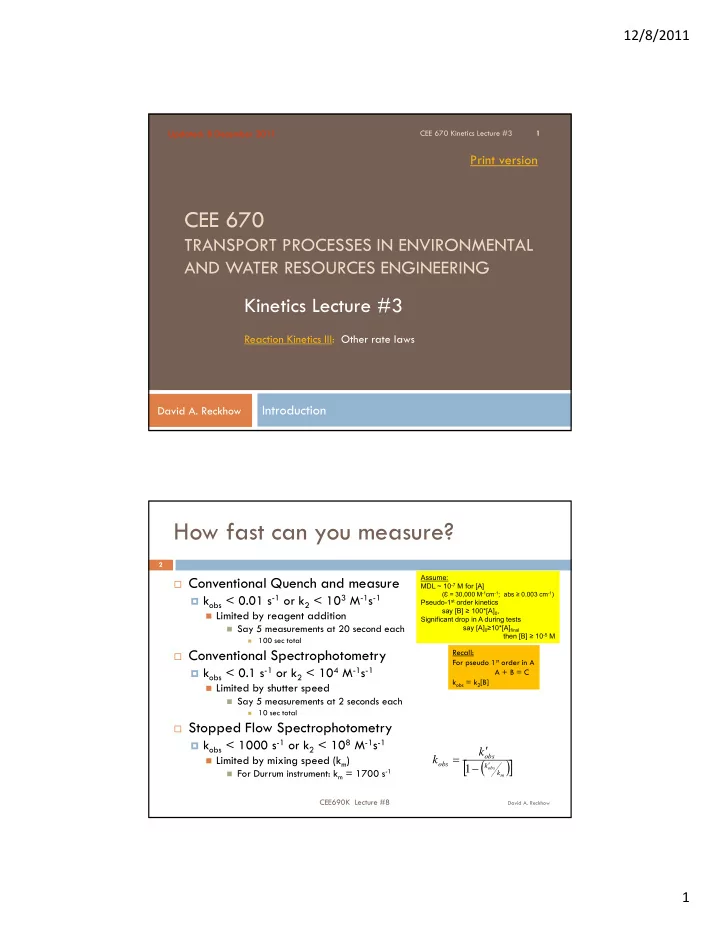
How fast can you measure?

David A. Reckhow

CEE690K Lecture #8

2

 Conventional Quench and measure  kobs < 0.01 s-1 or k2 < 103 M-1s-1  Limited by reagent addition

 Say 5 measurements at 20 second each

 100 sec total

 Conventional Spectrophotometry  kobs < 0.1 s-1 or k2 < 104 M-1s-1  Limited by shutter speed

 Say 5 measurements at 2 seconds each

 10 sec total

 Stopped Flow Spectrophotometry  kobs < 1000 s-1 or k2 < 108 M-1s-1  Limited by mixing speed (km)

 For Durrum instrument: km = 1700 s-1

   

m

• bs k

k

• bs
• bs

k k



   1

Assume: MDL ~ 10-7 M for [A] (Ɛ = 30,000 M-1cm-1; abs ≥ 0.003 cm-1) Pseudo-1st order kinetics say [B] ≥ 100*[A]0, Significant drop in A during tests say [A]0≥10*[A]final then [B] ≥ 10-5 M

Recall: For pseudo 1st order in A A + B = C kobs = k2[B]

12/8/2011 2

Do we care about fast reactions?

David A. Reckhow

CEE 670 Kinetics Lecture #2

3

 Competitive Kinetics  Selective contaminant destruction  Ethinylestradiol vs phenol  Direction for Byproduct Formation

O3

pH

2 4 6 8 10 12 14

Log 

• 12
• 10
• 8
• 6
• 4
• 2

alpha-HOCl alpha-phenate product of alphas

Alternative #1 for very fast reactions

David A. Reckhow

CEE 670 Kinetics Lecture #5

4

 Make use of known pH speciation of reactants  Pick conditions where “formal” concentrations are easily

measured, but reactive forms are orders of magnitude lower

 e.g., chlorination of phenol

products O H C HOCl

k

  



2

5 6

] [ ] [ ] [ ] [ ] [ ] ][ [

2 2 1 2 5 6 2    

     H K K phenol H K H chlorine k O H C HOCl k dt dc

a a tot a tot

] [ ] [ ] [ ] [ ] [

2 2 1 2   

   H K K H K H phenol chlorine k k

a a a tot tot

• bs

12/8/2011 3

pH

2 4 6 8 10 12 14

Log 

• 12
• 10
• 8
• 6
• 4
• 2

alpha-HOBr alpha-phenate product of alphas

Alt #1 example: Bromine + phenol

David A. Reckhow

CEE 670 Kinetics Lecture #5

5

 Flow injection analysis  Allowed 10-150 ms reaction

time

 Gallard et al., 2003

 Wat. Res. 379:2883

Alternative #2 for very fast reactions

David A. Reckhow

CEE 670 Kinetics Lecture #5

6

 Use competitive kinetics  Time drops out  just wait until “C” is gone  Must know one of the two rate constants (say kB), and

concentrations of both A & B (initial and final)

 So the accessible range for kA is roughly 0.2*kB to 5*kB

Q C B P C A

B A

k k

     

] ][ [ ] [ ] ][ [ ] [ C B k dt B d C A k dt A d

B A

   

                  

 

] [ ] [ ln ] [ ] [ ln ] [ ] [ ] [ ] [ ] [ ] [ ] [ ] [ B B k k A A B B d k k A A d B k A k B d A d

B A B A B A

12/8/2011 4

Alt #2 Example: bromine & phenols

David A. Reckhow

CEE 670 Kinetics Lecture #5

7

 HPLC determination of residual

phenols

 Acero et al., 2005  Wat. Res. 39:2979

Mixed Second Order

David A. Reckhow

CEE 670 Kinetics Lecture #2

8

 Two different reactants  Initial Concentrations are different; [A]0≠[B]0

 The integrated form is:  Which can be expressed as:

products B A

k

  

2

   dt A d dt d V rate

A

] [ 1 1  

  

x B x A k B A k dt dx    

2 2

] [ ] [ ] ][ [

t k B A A B B A

2

] [ ] [ ] [ ] [ ln ] [ ] [ 1    

2

] [ ] [ log ] [ ] [ 43 . ] [ ] [ log A B t B A k B A    ] [ ] [ log B A

t

] [ ] [ log B A

Similar to equ 9.18 in Clark

12/8/2011 5

Mixed Second Order

David A. Reckhow

CEE 670 Kinetics Lecture #2

9

 Initial Concentrations are the same; [A]0=[B]0

 The integrated form is:  Which can be integrated:

products B A

k

  

2

  

x A x A k A A k dt dx    

2 2

] [ ] [ ] ][ [

2

] [ 1 2 ] [ 1 A t k A   ] [ 1 A

t

] [ 1 A

x B x A B A      ] [ ] [ ] [ ] [

 

 dt k A A d

A 2 2

] [ ] [  t k A A

2

2 ] [ 1 ] [ 1  

David A. Reckhow

CEE 670 Kinetics Lecture #2

10

Pseudo first order

 For most reactions, n=1 for each of two different

reactants, thus a second-order overall reaction

1 1 2 B Ac

c k dt dc  

1 1 5

min 10 9 . 3

  

 Lmg x k

 Many of these will have one reactant in great excess (e.g., B)

 These become “pseudo-1st

• rder in the limiting reactant,

as the reactant in excess really doesn’t change in concentration

B

c

A

c

products B A

k

  

2

12/8/2011 6

10 20 30 40 50 60 70 80 90 20 40 60 80 Time (min) Concentration

David A. Reckhow

CEE 670 Kinetics Lecture #2

11

Pseudo-1st order (cont.)

 Since C2 changes little

from its initial 820 mg/L, it is more interesting to focus

• n CA

 CA exhibits simple 1st

• rder decay, called

pseudo-1st order

 The pseudo-1st order rate

constant is just the “observed rate” or kobs

1 1 2 B Ac

c k dt dc  

t k Ao A

• bs

e c c





1 5 2

min 032 . ) 820 ( 10 9 . 3

 

   x c k k

B

• bs

Example: O3 & Naphthalene

David A. Reckhow

CEE 670 Kinetics Lecture #2

12

 How long will it take for ozone (4.8

mg/L dose) to reduce the concentration of naphthalene by 99%?

 Used in moth balls and as a chemical

intermediate

 2nd order reaction; k2 = 3000 M-1s-1

 Table 1 in Hoigne & Bader, 1983 [Wat.

• Res. 17:2:173]

 Industrial WW with 0.1mM naphthalene

 Both reactants are at same (0.1mM)

concentration

 Therefore, this reduces to a simple 2nd

• rder reaction

t k A A

2

] [ 1 ] [ 1   t 3000 10 1 10 1

4 6

 

 

min 5 . 5 sec 330 000 , 990 3000    t t

12/8/2011 7

O3 & Naphthalene (cont.)

David A. Reckhow

CEE 670 Kinetics Lecture #2

13

 Contaminated river water (0.001 mM)  Now ozone is in great molar excess, so this is a pseudo-1st

• rder reaction

t B k

e A A

2

] [

] [ ] [





 

 

sec 4 . 15 3 . 605 . 4 10 3000 10 10 ln ] [ ] [ ] [ ln

4 6 8 2

             

  

t t t t B k A A

Molecularity of three: 3rd order kinetics

David A. Reckhow

CEE 670 Kinetics Lecture #2

14

 Quite improbably, but sometimes happens  Three different reactants  Complicated integrated form exists  Two different reactants  Integrated form:

products C B A

k

   

3

   

x C x B x A k C B A k dt dx     

3 3

] [ ] [ ] [ ] ][ ][ [

products B A

k

  

3

2

   

x B x A k B A k dt dx    

2 3 2 3

] [ 2 ] [ ] [ ] [

    

t k A B B A A B A A A B A A

3 2

] [ ] [ 2 ] [ ] [ ] [ ] [ ln ] [ ] [ ] [ ] [ 2 ] [ ] [     

12/8/2011 8

3rd Order (cont.)

David A. Reckhow

CEE 670 Kinetics Lecture #2

15

 Only one reactant or Initial Concentrations are the same

 The integrated form is:  Which can be integrated:

products A

k

  3 3

   

x A x A x A k A A A k dt dx     

3 3

] [ ] [ ] [ ] ][ ][ [

2 3 2

] [ 1 6 ] [ 1 A t k A  

2

] [ 1 A

t

2

] [ 1 A

 

 dt k A A d

A 3 3

] [ ] [  t k t k A A

A 3 3 2 2

6 2 ] [ 1 ] [ 1     

3rd Order (cont.)

David A. Reckhow

CEE 670 Kinetics Lecture #2

16

 Pseudo-2nd order reactions  When one of the reactants has a fixed concentration

 E.g., present in excess or buffered, or acts catalytically

 Like a regular 2nd order reaction with two reactants but

• bserved constant is fundamental rate constant times

concentration of the 3rd reactant.

 The integrated form:

t C k B A A B B A ] [ ] [ ] [ ] [ ] [ ln ] [ ] [ 1

3

 

• bs

k

12/8/2011 9

Example: chlorate formation

David A. Reckhow

CEE 670 Kinetics Lecture #2

17

 Formation of chlorate in concentrated hypochlorite

solutions

 Concern: chlorate is toxic  MCLG=0.2 mg/L  Stoichiometry  Is this 3rd order? Be skeptical!  Observed kinetics  So, why is it 2nd order?

  

  Cl ClO OCl 2 3

3

 

2 3 ]

[

 

 OCl k dt ClO d

• bs

Chlorate example (cont.)

David A. Reckhow

CEE 670 Kinetics Lecture #2

18

 Answer: this is a reaction pathway composed of two

elementary reactions

 Step #1  Step #2  In multi-step reactions such as these, we say that  the overall rate is determined by the slowest step

 Called the “rate-limiting step” or RLS

 Rate law is written based on the RLS  Subsequent steps are ignored  Prior steps are incorporated as they determine the

concentrations of the RLS reactants

  

    Cl ClO OCl

slow 2

2

   

     Cl ClO ClO OCl

fast 3 2

H

12/8/2011 10

David A. Reckhow

CEE 670 Kinetics Lecture #2

19

Reversible reaction kinetics

For a general reversible reaction:

k qQ + pP bB + aA k

r f



And the rate law must consider both forward and reverse reactions:

where, kf = forward rate constant, [units depend on a and b] kb or kr = backward rate constant, [units depend on a and b] CP = concentration of product species P, [moles/liter] CQ = concentration of product species Q, [moles/liter] p = stoichiometric coefficient of species P q = stoichiometric coefficient of species Q

q Q p P r b B a A f

C C k C C k rate  

David A. Reckhow

CEE 670 Kinetics Lecture #2

20 Reversible 1st order reactions

Stumm & Morgan

• Fig. 2.10
• Pg. 69

] [ ] [

2 1

B k A k dt dB  

eq

K k k A B B k A k dt dB     

2 1 2 1

] [ ] [ ] [ ] [

 Kinetic law  Eventually the reaction

slows and,

 Reactant concentrations

approach the equilibrium values

12/8/2011 11

Reversible 1st order (cont.)

David A. Reckhow

CEE 670 Kinetics Lecture #2

21

 Solution to non-equilibrium reaction period  See Brezonik, pg 37-38 for details  Where k* = kf + kr  And:  Where:

 

t k f r

e k k A k A

*

*

] [ 1 ] [



 

k P A k

r f



t k equ equ

e A A A A

*

] [ ] [ ] [ ] [



  

 

equ equ equ r f

A P K k k ] [ ] [  

Linearized version

Equivalent to equ 9.60 in Clark

David A. Reckhow

CEE 670 Kinetics Lecture #3

22

 To next lecture