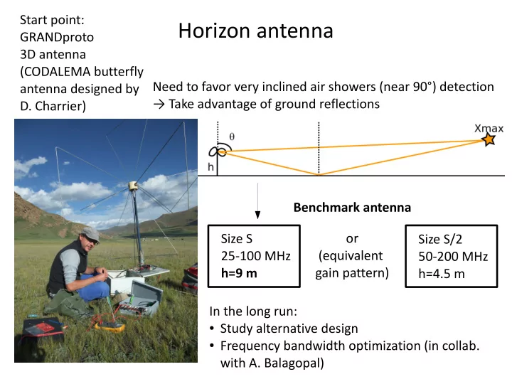
SLIDE 1 Horizon antenna
Need to favor very inclined air showers (near 90°) detection → Take advantage of ground reflections Size S 25-100 MHz h=9 m Size S/2 50-200 MHz h=4.5 m Start point: GRANDproto 3D antenna (CODALEMA butterfly antenna designed by
(equivalent gain pattern) Benchmark antenna In the long run:
- Study alternative design
- Frequency bandwidth optimization (in collab.
with A. Balagopal)
SLIDE 2
Antenna gain pattern
G(q,j): unloaded butterfly antenna X-arm response to q,j wave @ 50 MHz NEC4 simulation wih infinite ground (“sandy dry”) hypothesis → G = 0 @ q >= 90°, huge gradiant (<-18dB between 80 & 90°), effect of infinite ground simulation Symmetrical pattern for j > 90°
SLIDE 3
Infinite ground Soil Mesh over soil
Antenna gain pattern
Effect of a realistic ground (simulation) G > 0 @ q >= 90° SKALA antenna, H plane, 150 MHz (from SKA paper)
https://arxiv.org/ftp/arxiv/papers/1512/1512.01453.pdf
q
SLIDE 4 Antenna orientation
a,b, angles of ground normal vector (=antenna pole) in GRAND frame computed from topography with 30 m step data
- Antenna X-arm and Y-arm // to ground
- Projection of X-arm and Y-arm on XY plane along NS & EW
X-arm Y-arm
SLIDE 5
Antenna orientation
If antenna pole is not put ^ to ground → arms are not // to ground → antenna response does not differ much for q in 80-90° 75 MHz 125 MHz 175 MHz 18° tilt ^ to ground
SLIDE 6 GRAND frame to antenna frame
- Hyp. : all radio emission comes from Xmax position
→ calculation of Xmax direction in antenna frame (qant,jant) to apply antenna response
SLIDE 7
Antenna voltage response
Vpp EW Vpp NS~0 Vpp UP V=Leq(n,q,j).E Leq: equivalent length of antenna connected to a circuit RLC (300 W, 6.5e-12 F, 1e-6 H )
SLIDE 8 Events selection
Stationnary noise @ 50-200 MHz
- Ground: T ~ 290 K black body
- Sky: LFmap (galaxy..) T(direction, LST)
Atmosphere T ~ 0 K
→ Selected air shower event if Pessimistic (conservative) hyp. 8+ antennas with Vpp > 10 Vrms(noise) Optimistic (agressive) hyp. 5+ antennas with Vpp > 3 Vrms(noise) & antennas are selected if not isolated: distance to 1+ other selected antenna(s) < 2 antenna array step Vpp > 10 Vrms Add noise + digitization of V
SLIDE 9
t events simulation
Hotspot 500 m step antenna array ~ 10 000 km² Decay positions of t (weighted by Waxman-Bahcall 1/3 nt flux) 20 000 (detectable) t events are simulated, between 1017 to 1021 eV
SLIDE 10 antenna array ~ 10 000 km² antennas in the 3° light cone holes ↔ mountain shadowing
EW
antennas with a computed voltage additional holes ↔ qant (Xmax ) > 89.5° array step = 500m
t event example
SLIDE 11
Ground slope affects voltage
a = zenithal angle (deg) of ground normal vector qant = Xmax zenithal angle in antenna frame Vpp = f(qant) & qant = f(a) Vpp (µV) Big differences of a for nearby antennas: calculation of a from 30m step topography not accurate → Limitation for Vpp computation accuracy
SLIDE 12
Optimistic hyp. 1000 m step array
t events simulation
Number of antennas per shower Not in moutain shadow With a computed voltage Which triggers on Vpp condition
SLIDE 13
Exposure
Agressive = Optimistic hyp. Conservative = Pessimistic hyp. As expected, conservative hyp. (8+ antennas with Vpp > 10 Vrms(noise) ) cuts a lot of low energy events, but keeps half of high energy events Preliminary study and new study compatible
SLIDE 14
Exposure
Agressive = Optimistic hyp. Conservative = Pessimistic hyp. 500 m step array: density = 4 ant / km² Density *4 Exposure ~*2 1500 m step array density = 0.44 ant / km² Density /2.3 Exposure ~/2 100m step array: density = 1 ant / km²
SLIDE 15 t detection rate
- Prelim. study optimistic: 2.8 yr-1
500 m light cone: 7.568 +-0.097 yr-1 500 m optimistic: 2.975 +-0.032 yr-1 500 m pessimistic: 0.807 +-0.008 yr-1 1000 m optimistic: 1.490 +-0.021 yr-1 1000 m pessimistic: 0.299 +-0.004 yr-1 1500 m optimistic: 0.720 +-0.009 yr-1 1500 m pessimistic: 0.118 +-0.001 yr-1 t detection rate (yr-1) = exposure (1 yr) * flux * dE flux = Waxman-Bahcall, 1/3 nt = 2e-4 /3 * E-2 GeV-1.m-2.sr-1.s-1
SLIDE 16
t detection rate (decay positions)
antenna array ~ 10 000 km² Optimistic hyp. 1000 m step array
SLIDE 17 t detection rate (directions)
downgoing upgoing To South To South To North Optimistic hyp. 1000 m step array
- We might get more upgoing events with a proper ground in the simulation
- f antenna response
- t events mainly come from North (they travel towards South) because
Southern ridge of Tianshan mountains act as target for neutrino decays
SLIDE 18 Conclusion & to do
- Results of new simulation compatible
with preliminary simulation
- Improvements on exposure depend on
antenna design and its fair simulation
- Comparison with a flat array to quantify topography effects
- Comparison with a real topography array but with vertical antennas to quantify
the effect of the antenna response
- Simulation for arrays in the whole Western China (to be done for March 2018)
- Find a way to simulate antenna response with a realistic ground (HFSS?)
To do Conclusion