Homology Modeling I Basel, September 30, 2004 Torsten Schwede - PDF document

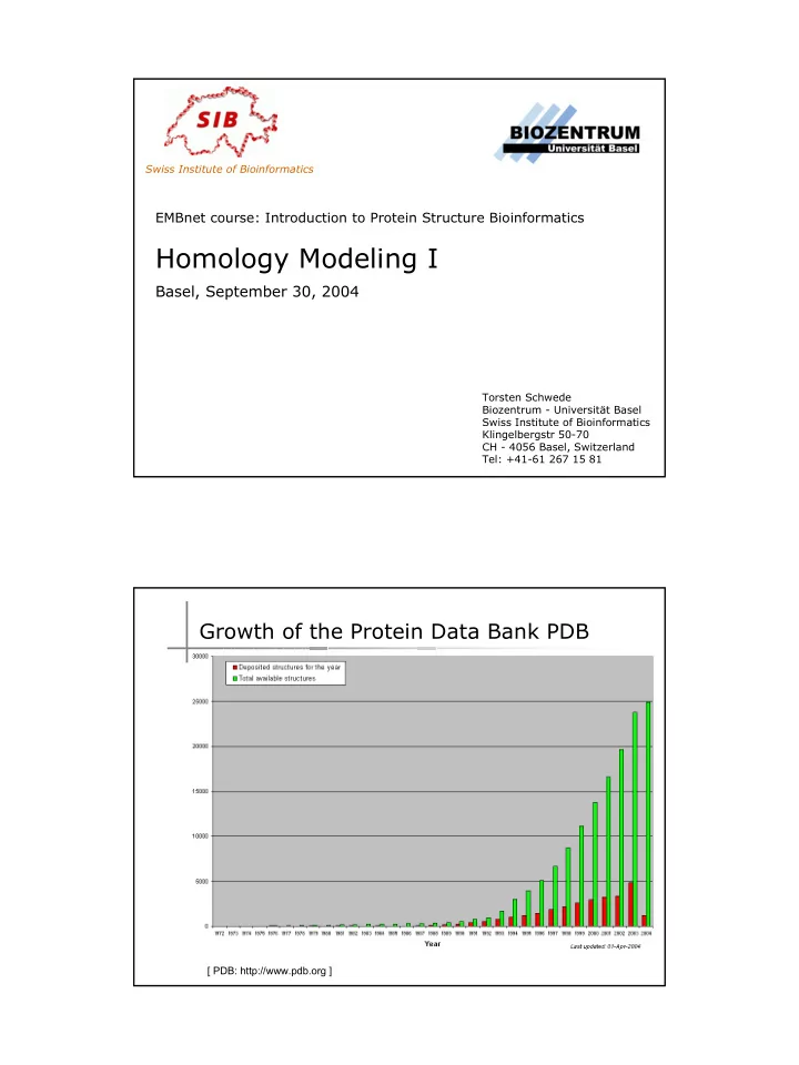
Swiss Institute of Bioinformatics EMBnet course: Introduction to Protein Structure Bioinformatics Homology Modeling I Basel, September 30, 2004 Torsten Schwede Biozentrum - Universität Basel Swiss Institute of Bioinformatics Klingelbergstr 50-70 CH - 4056 Basel, Switzerland Tel: +41-61 267 15 81 Growth of the Protein Data Bank PDB [ PDB: http://www.pdb.org ]

Public Database Holdings 1'000'000 � No experimental structure for most 100'000 sequences 10'000 TrEMBL 1'000 SwissProt PDB 100 1986 1988 1990 1992 1994 1996 1998 2000 2002 2004 MNIFEMLRID EGLRLKIYKD TEGYYTIGIG HLLTKSPSLN AAKSELDKAI GRNCNGVITK DEAEKLFNQD VDAAVRGILR NAKLKPVYDS LDAVRRCALI NMVFQMGETG VAGFTNSLRM LQQKRWDEAA VNLAKSRWYN QTPNRAKRVI TTFRTGTWDA YKNL � Many proteins fold spontaneously to their native structure � Protein folding is relatively fast (nsec – sec) � Chaperones speed up folding, but do not alter the structure The protein sequence contains all information needed to create a correctly folded protein. Can we predict protein structures from protein sequences alone ( ab initio ) ?

Molecular Dynamics 2 k ( ) ∑ ν = − i l l i i , 0 2 bonds 2 k ( ) ∑ + θ − θ i i i , 0 2 angles V ( ( ) ) ∑ + + ω − γ N 1 cos n 2 torsions     12 6     σ σ q q N N   ∑ ∑       ij ij i j + πε − + 4       ij   πε  r r 4 r      = = + i 1 j i 1    ij ij 0 ij  Ab initio protein folding simulation 10 –4 seconds Physical time for simulation 10 –15 seconds Typical time-step size Number of MD time steps 10 11 Atoms in a typical protein and water simulation 32’000 Approximate number of interactions in force calculation 10 9 Machine instructions per force calculation 1000 Total number of machine instructions 10 23 BlueGene capacity (floating point operations per second) 1 petaflop (10 15 ) � Blue Gene will need 1-3 years to simulate 100 µ sec. [ http://www.research.ibm.com/bluegene/ ]

Rosetta Stone Approach � David Baker group � Find sequence patterns that strongly correlate with protein structure at the local level to create a library of fragments (I- sites). � E.g. „amphipathic helix“: Amino acid statistics Helix position Rosetta Stone Approach To build a model building for a new sequence: � Search for compatible fragments (reduced alphabet) � � Use Monte Carlo simulated annealing to assemble overlapping fragments Scoring functions are used to select best models (~1000) � http://isites.bio.rpi.edu

Rosetta Stone Approach Generates thousands of models � Best Models in CASP4: ~ 5 – 10 Å rmsd Ca � Difficult to distinguish good and bad models � http://isites.bio.rpi.edu The number of different protein folds is limited: Already known folds PDB submissions per year New folds Year

Evolution of the globin family: Evolution of protein structure families Rmsd of backbone atoms in core 2.5 2.0 1.5 1.0 0.5 0.0 100 50 0 Percent identical residues in core [ Chothia & Lesk (1986) ] � Common core = all residues that can be superposed in 3D � For proteins > 60% identical residues, the core contains > 90 % of all residues deviating less than 1.0 Å.

Sequence similarity implies structural similarity? 100 . ide ntity 80 Percentage sequence identity/similarity Sequence identity 60 implies structural similarity 40 Don’t know 20 region ..... 0 (B.Rost, Columbia, NewYork) 0 50 100 150 200 250 Number of residues aligned Sequence similarity implies structural similarity? 100 . ide ntity sim ila rity 80 Percentage sequence identity/similarity Sequence identity 60 implies structural similarity 40 Don’t 20 know region ..... 0 (B.Rost, Columbia, NewYork) 0 50 100 150 200 250 Number of residues aligned

Similar Sequence � Similar Structure Homology modeling = Comparative protein modeling = Knowledge-based modeling Idea: Using experimental 3D-structures of related family members (templates) to calculate a model for a new sequence (target). Comparative Modeling Known Structures (Templates) Target Template Selection Sequence Alignment Structure Evaluation & Template - Target Assessment Structure modeling Homology Model(s)

Comparative Modeling Known Structures (Templates) Target Template Selection Sequence Alignment Structure Evaluation & Template - Target Assessment • Protein Data Bank PDB http://www.pdb.org Structure modeling Homology Model(s) Database of templates � • Separate into single chains • Remove bad structures (models) • Create BLASTable database or fold library (profiles, HMMs) Comparative Modeling Known Structures (Templates) Target Template Selection Sequence Template selection: Alignment Structure Evaluation & Template - Target Assessment 1. Sequence Similarity / Fold Structure modeling recognition Homology Model(s) 2. Structure quality (resolution, experimental method) 3. Experimental conditions (ligands and cofactors)

Comparative Modeling Known Structures (Templates) Target Template Selection Sequence Alignment Structure Evaluation & Template - Target Assessment • Multiple sequence alignment for pairs > 40% identity Structure modeling or Homology Model(s) • Use structural alignment of templates to guide sequence alignment of target or • Use separate profiles for template and targets Comparative Modeling Known Structures (Templates) Target Template Selection Sequence Alignment Structure Evaluation & Template - Target Assessment • Errors in template selection or Structure modeling alignment result in bad models Homology Model(s) iterative cycles of alignment, � modeling and evaluation Built many models, � choose best.

Comparative Modeling Known Structures (Templates) Target Template Selection Sequence Alignment Structure Evaluation & Template - Target Assessment I. Manual Model building Structure modeling Homology II. Template based fragment Model(s) assembly – Composer (Sybyl, Tripos) – SWISS-MODEL III. Satisfaction of spatial restraints – Modeller (Insight II, MSI) – CPH-Models I. Manual Modeling [ http://www.expasy.org/spdbv/ ]

II. Template based fragment assembly � Find structurally conserved core regions II. Template based fragment assembly Build model core � � … by averaging core template backbone atoms (weighted by local sequence similarity with the target sequence). Leave non-conserved regions (loops) for later ….

II. Template based fragment assembly � Loop (insertion) modeling � Use the “spare part” algorithm to find compatible fragments in a Loop- Database, or “ab-initio” rebuilding (e.g. Monte Carlo, MD, GA, etc.) to build missing loops. II. Template based fragment assembly � Side Chain placement � Find the most probable side chain conformation, using • homologues structure information • back-bone dependent rotamer libraries • energetic and packing criteria

II. Template based fragment assembly � Rotamer Libraries � Only a small fraction of all possible side chain conformations is observed in experimental structures � Rotamer libraries provide an ensemble of likely conformations � The propensity of rotamers depends on the backbone geometry: Backbone-dependent rotamer libraries p(g+ | psi) Phe,Tyr, His p(g+ | phi) g+ p(t | phi) p(t | psi) trans p(g- | psi) p(g- | phi) g-

II. Template based fragment assembly � Energy minimization � modeling method will produce unfavorable contacts and bonds � Energy minimization is used to • regularize local bond and angle geometry • Relax close contacts and geometric strain � extensive energy minimization will move coordinates away from real structure ⇒ keep it to a minimum � SWISS-MODEL is using GROMOS 96 force field for a steepest descent III. Satisfaction of Spatial restraints � Alignment of target sequence with templates � Extraction of spatial restraints from templates � Modeling by satisfaction of spatial restraints Q M T S A F G T A E

III. Satisfaction of Spatial restraints Some features of a protein structure: R resolution of X-ray experiment r amino acid residue type Φ , Ψ main chain angles t secondary structure class M main chain conformation class Χ i, , c i side chain dihedral angle class a residue solvent accessibility s residue neighborhood difference d C a - C a distance ∆ d difference between two C a - C a distances III. Satisfaction of Spatial restraints � Feature properties can be associated with � a protein (e.g. X-ray resolution) � residues (e.g. solvent accessibility) � pairs of residues (e.g. C a - C a distance) � other features (e.g. main chain classes) � How can we derive modeling restraints from this data? � A restraint is defined as probability density function ( pdf ) p(x): ∫ = x 1 p ( x ) dx 1 ∫ ≤ < = p ( x 1 x x 2 ) p ( x ) dx with x 2 > p ( x ) 0