Hoare Logic and Model Checking These slides are heavily based on - - PowerPoint PPT Presentation

▶

Nov 20, 2022 112 likes •869 views

Acknowledgements Hoare Logic and Model Checking These slides are heavily based on previous versions by Mike Gordon, Alan Mycroft, and Kasper Svendsen. Jean Pichon-Pharabod University of Cambridge Thanks to Mistral Contrastin, Victor Gomes, Joe

SLIDE 1

Hoare Logic and Model Checking

Jean Pichon-Pharabod University of Cambridge CST Part II – 2017/18

Acknowledgements

These slides are heavily based on previous versions by Mike Gordon, Alan Mycroft, and Kasper Svendsen. Thanks to Mistral Contrastin, Victor Gomes, Joe Isaacs, Ian Orton, and Domagoj Stolfa for reporting mistakes.

Motivation

We often fail to write programs that meet our expectations, which we phrased in their specifications:

we fail to write programs that meet their specification;
we fail to write specifications that meet our expectations.

Addressing the former issue is called verification, and addressing the latter is called validation.

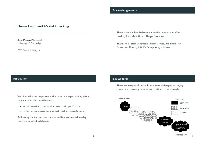
Background

There are many verification & validation techniques of varying coverage, expressivity, level of automation, ..., for example: typing testing model checking program logics

perational

reasoning expressivity automation coverage: complete bounded sparse

SLIDE 2

Choice of technique

More expressive and complete techniques lead to more confidence. It is important to choose the right set of verification & validation techniques for the task at hand:

verified designs may still not work;
verification can give a false sense of security;
verification can be very expensive and time-consuming.

More heavyweight techniques should be used together with testing, not as a replacement.

Course structure

This course is about two techniques, their underlying ideas, how to use them, and why they are correct:

Hoare logic (Lectures 1-6);
Model checking (Lectures 7-12).

These are not just techniques, but also ways of thinking about programs.

Lecture plan

Lecture 1: Informal introduction to Hoare logic Lecture 2: Formal semantics of Hoare logic Lecture 3: Examples, loop invariants, and total correctness Lecture 4: Mechanised program verification Lecture 5: Separation logic Lecture 6: Examples in separation logic

Hoare logic

SLIDE 3

Hoare logic

Hoare logic is a formalism for relating the initial and terminal state of a program. Hoare logic was invented in 1969 by Tony Hoare, inspired by earlier work of Robert Floyd. There was little-known prior work by Alan Turing. Hoare logic is still an active area of research.

Partial correctness triples

Hoare logic uses partial correctness triples (also “Hoare triples”) for specifying and reasoning about the behaviour of programs: {P} C {Q} is a logical statement about a command C, where P and Q are state predicates:

P is called the precondition, and describes the initial state;
Q is called the postcondition, and describes the terminal state.

Components of a Hoare logic

To define a Hoare logic, we need four main components:

the programming language that we want to reason about:

its syntax and dynamic (e.g. operational) semantics;

an assertion language for defining state predicates:

its syntax and an interpretation;

an interpretation of Hoare triples;
a (sound) syntactic proof system for deriving Hoare triples.

This lecture will introduce each component informally. In the coming lectures, we will cover the formal details.

The WHILE language

SLIDE 4

Commands of the WHILE language

WHILE is the prototypical imperative language. Programs consist

f commands, which include branching, iteration, and assignment:

C ::= skip | C1; C2 | V := E | if B then C1 else C2 | while B do C Here, V is a variable, E is an arithmetic expression, which evaluates to an integer, and B is a boolean expression, which evaluates to a boolean. States are mappings from variables to integers.

Expressions of the WHILE language

The grammar for arithmetic expressions and boolean expressions includes the usual arithmetic operations and comparison operators, respectively: E ::= N | V | E1 + E2 arithmetic expressions | E1 − E2 | E1 × E2 | · · · B ::= T | F | E1 = E2 boolean expressions | E1 ≤ E2 | E1 ≥ E2 | · · · Note that expressions do not have side effects.

Assertions and specifications

The assertion language

Assertions (also “state predicates”) P, Q, . . . include boolean expressions (which can contain program variables), combined using the usual logical operators: ∧, ∨, ¬, ⇒, ∀, ∃, . . . For instance, the predicate X = Y + 1 ∧ Y > 0 describes states in which the variable Y contains a positive value, and the value of X is equal to the value of Y plus 1.

SLIDE 5

Informal semantics of partial correctness triples

The partial correctness triple {P} C {Q} holds if and only if:

assuming C is executed in an initial state satisfying P,
and assuming moreover that this execution terminates,
then the terminal state of the execution satisfies Q.

For instance,

{X = 1} X := X + 1 {X = 2} holds;
{X = 1} X := X + 1 {X = 3} does not hold.

Partial correctness

Partial correctness triples are called partial because they only specify the intended behaviour of terminating executions. For instance, {X = 1} while X > 0 do X := X + 1 {X = 0} holds, because the given program never terminates when executed from an initial state where X is 1. Hoare logic also features total correctness triples that strengthen the specification to require termination.

Informal semantics of total correctness

There is no standard notation for total correctness triples; we will use [P] C [Q]. The total correctness triple [P] C [Q] holds if and only if:

assuming C is executed in an initial state satisfying P,
then the execution terminates,
and the terminal state satisfies Q.

Total correctness

The following total correctness triple does not hold: [X = 1] while X > 0 do X := X + 1 [X = 0]

the loop never terminates when executed from an initial state

where X is positive. The following total correctness triple does hold: [X = 0] while X > 0 do X := X + 1 [X = 0]

the loop always terminates immediately when executed from

an initial state where X is zero.

SLIDE 6

Total correctness, partial correctness, and termination

Informally: total correctness = partial correctness + termination. It is often easier to show partial correctness and termination separately. Termination is usually straightforward to show, but there are examples where it is not: no one knows whether the program below terminates for all values of X: while X > 1 do if ODD(X) then X := 3 × X + 1 else X := X DIV 2 Microsoft’s T2 tool is used to prove termination of systems code.

Examples of specifications

Corner cases of partial correctness triples

{⊥} C {Q}

this says nothing about the behaviour of C,

because ⊥ never holds for any initial state. {⊤} C {Q}

this says that whenever C halts, Q holds.

{P} C {⊤}

this holds for every precondition P and command C,

because ⊤ always holds in the terminate state.

Corner cases of total correctness triples

[P] C [⊤]

this says that C always terminates when executed from an

initial state satisfying P. [⊤] C [Q]

this says that C always terminates, and ends up in a state

where Q holds.

SLIDE 7

The need for auxiliary variables

How can we specify that a program C computes the maximum of two variables X and Y , and stores the result in a variable Z? Is this a good specification for C? {⊤} C {(X ≤ Y ⇒ Z = Y ) ∧ (Y ≤ X ⇒ Z = X)} No! Take C to be X := 0; Y := 0; Z := 0 Then C satisfies the above specification! The postcondition should refer to the initial values of X and Y .

Auxiliary variables

In Hoare logic, we use auxiliary variables (also “ghost variables”,

r “logical variables”), which are not allowed not occur in the

program, to refer to the initial values of variables in postconditions. Notation: program variables are uppercase, and auxiliary variables are lowercase. v ranges over auxiliary variables, and concrete values are x, y, . . .. For instance, {X = x ∧ Y = y} C {X = y ∧ Y = x} expresses that if C terminates, then it exchanges the values of variables X and Y .

Formal proof system for Hoare logic

Hoare logic

We will now introduce a natural deduction proof system for partial correctness triples due to Tony Hoare. The logic consists of a set of inference rule schemas for deriving consequences from premises. If S is a statement, we will write ⊢ S to mean that the statement S is derivable. We will have two derivability judgements:

⊢ P, for derivability of assertions; and
⊢ {P} C {Q}, for derivability of partial correctness triples.

SLIDE 8

Inference rule schemas

The inference rule schemas of Hoare logic will be specified as follows: ⊢ S1 · · · ⊢ Sn ⊢ S This expresses that S may be deduced from assumptions S1, ..., Sn. These are schemas that may contain meta-variables.

Proof trees

A proof tree for ⊢ S in Hoare logic is a tree with ⊢ S at the root, constructed using the inference rules of Hoare logic, where all nodes are shown to be derivable (so leaves require no further derivations): ⊢ S1 ⊢ S2 ⊢ S3 ⊢ S4 ⊢ S We typically write proof trees with the root at the bottom.

Formal proof system for Hoare logic

⊢ {P} skip {P} ⊢ {P[E/V ]} V := E {P} ⊢ {P} C1 {Q} ⊢ {Q} C2 {R} ⊢ {P} C1; C2 {R} ⊢ {P ∧ B} C1 {Q} ⊢ {P ∧ ¬B} C2 {Q} ⊢ {P} if B then C1 else C2 {Q} ⊢ {P ∧ B} C {P} ⊢ {P} while B do C {P ∧ ¬B} ⊢ P1 ⇒ P2 ⊢ {P2} C {Q2} ⊢ Q2 ⇒ Q1 ⊢ {P1} C {Q1}

The skip rule

⊢ {P} skip {P} The skip rule expresses that any assertion that holds before skip is executed also holds afterwards. P is a meta-variable ranging over an arbitrary state predicate. For instance, ⊢ {X = 1} skip {X = 1}.

SLIDE 9

The assignment rule

⊢ {P[E/V ]} V := E {P} Here, P[E/V ] means the assertion P with the expression E substituted for all occurrences of the variable V . For instance, ⊢ {X + 1 = 2} X := X + 1 {X = 2} ⊢ {Y + X = Y + 10} X := Y + X {X = Y + 10}

The assignment rule

The assignment rule reads right-to-left; could we use another rule that reads more easily? Consider the following plausible alternative assignment rule: ⊢ {P} V := E {P[E/V ]} We can instantiate this rule to obtain the following triple, which does not hold: {X = 0} X := 1 {1 = 0}

The rule of consequence

⊢ P1 ⇒ P2 ⊢ {P2} C {Q2} ⊢ Q2 ⇒ Q1 ⊢ {P1} C {Q1} The rule of consequence allows us to strengthen preconditions and weaken postconditions. Note: the ⊢ P ⇒ Q hypotheses are a different kind of judgment. For instance, from ⊢ {X + 1 = 2} X := X + 1 {X = 2}, we can deduce ⊢ {X = 1} X := X + 1 {X = 2}.

Sequential composition

⊢ {P} C1 {Q} ⊢ {Q} C2 {R} ⊢ {P} C1; C2 {R} If the postcondition of C1 matches the precondition of C2, we can derive a specification for their sequential composition. For example, if we have deduced:

⊢ {X = 1} X := X + 1 {X = 2}
⊢ {X = 2} X := X × 2 {X = 4}

we may deduce that ⊢ {X = 1} X := X + 1; X := X × 2 {X = 4}.

SLIDE 10

The conditional rule

⊢ {P ∧ B} C1 {Q} ⊢ {P ∧ ¬B} C2 {Q} ⊢ {P} if B then C1 else C2 {Q} For instance, to prove that ⊢ {⊤} if X ≥ Y then Z := X else Z := Y {Z = max(X, Y )} it suffices to prove that ⊢ {⊤ ∧ X ≥ Y } Z := X {Z = max(X, Y )} and ⊢ {⊤ ∧ ¬(X ≥ Y )} Z := Y {Z = max(X, Y )}.

The loop rule

⊢ {P ∧ B} C {P} ⊢ {P} while B do C {P ∧ ¬B} The loop rule says that

if P is an invariant of the loop body when the loop condition

succeeds, then P is an invariant for the whole loop, and

if the loop terminates, then the loop condition failed.

We will return to be problem of finding loop invariants.

(Redundant) Conjunction and disjunction rules

⊢ {P1} C {Q} ⊢ {P2} C {Q} ⊢ {P1 ∨ P2} C {Q} ⊢ {P} C {Q1} ⊢ {P} C {Q2} ⊢ {P} C {Q1 ∧ Q2} These rules are useful for splitting up proofs. Any proof with these rules could be done without using them

i.e. they are theoretically redundant (proof omitted),
however, they are useful in practice.

Summary

Hoare logic is a formalism for reasoning about the behaviour of programs by relating their initial and terminal state. It uses an assertion logic based on first-order logic to reason about program states, and extends this with Hoare triples to reason about the programs. Papers of historical interest:

C. A. R. Hoare. An axiomatic basis for computer
programming. 1969.
R. W. Floyd. Assigning meanings to programs. 1967.
A. M. Turing. Checking a large routine. 1949.

In the next lecture, we will formalise the intuitions we gave today, and prove soundness of Hoare logic.

SLIDE 11

Hoare logic

Lecture 2: Formalising the semantics of Hoare logic

Jean Pichon-Pharabod University of Cambridge CST Part II – 2017/18

Semantics of Hoare logic

Recall: to define a Hoare logic, we need four main components:

the programming language that we want to reason about:

its syntax and dynamic semantics;

an assertion language for defining state predicates:

its syntax and an interpretation;

an interpretation of Hoare triples;
a (sound) syntactic proof system for deriving Hoare triples.

This lecture defines a formal semantics of Hoare logic, and introduces properties of Hoare logic (soundness & completeness).

Dynamic semantics of WHILE

SLIDE 12

Dynamic semantics of WHILE

The dynamic semantics of WHILE will be given in the form of a “big-step” operational semantics. The reduction relation, written C, s ⇓ s′, expresses that the command C reduces to the terminal state s′ when executed from initial state s.

Dynamic semantics of WHILE

More precisely, these “states” are stacks, which are functions from variables to integers: s ∈ Stack

def

= Var → Z These are total functions, and define the current value of every program variable and auxiliary variable. This models WHILE with arbitrary precision integer arithmetic. A more realistic model might use 32-bit integers and require reasoning about overflow, etc.

Dynamic semantics of WHILE

The reduction relation is defined inductively by a set of inference rule schemas. To reduce an assignment, we first evaluate the expression E using the current stack, and update the stack with the value of E: E[ [E] ](s) = N V := E, s ⇓ s[V → N] We use functions E[ [E] ](s) and B[ [B] ](s) to evaluate arithmetic expressions and boolean expressions in a given stack s, respectively. For example, if s(X) = 3, then E[ [X + 2] ](s) = 5, so Y := X + 2, s ⇓ s[Y → 5].

Semantics of expressions

E[ [E] ](s) evaluates arithmetic expression E to an integer in stack s: E[ [−] ](=) : Exp × Stack → Z E[ [N] ](s)

def

= N E[ [V ] ](s)

def

= s(V ) E[ [E1 + E2] ](s)

def

= E[ [E1] ](s) + E[ [E2] ](s) . . . This semantics is too simple to handle operations such as division, which fails to evaluate to an integer on some inputs. For example, if s(X) = 3 and s(Y ) = 0, then E[ [X + 2] ](s) = E[ [X] ](s) + E[ [2] ](s) = 3 + 2 = 5, and E[ [Y + 4] ](s) = E[ [Y ] ](s) + E[ [4] ](s) = 0 + 4 = 4.

SLIDE 13

Semantics of boolean expressions

B[ [B] ](s) evaluates boolean expression B to a boolean in stack s: B[ [−] ](=) : BExp × Stack → B B[ [T] ](s)

def

= ⊤ B[ [F] ](s)

def

= ⊥ B[ [E1 ≤ E2] ](s)

def

=    ⊤ if E[ [E1] ](s) ≤ E[ [E2] ](s) ⊥

therwise

. . . For example, if s(X) = 3 and s(Y ) = 0, then B[ [X + 2 ≥ Y + 4] ](s) = E[ [X + 2] ](s) ≥ E[ [Y + 4] ](s) = 5 ≥ 4 = ⊤.

Big-step operational semantics of WHILE

E[ [E] ](s) = N V := E, s ⇓ s[V → N] C1, s ⇓ s′ C2, s′ ⇓ s′′ C1; C2, s ⇓ s′′ B[ [B] ](s) = ⊤ C1, s ⇓ s′ if B then C1 else C2, s ⇓ s′ B[ [B] ](s) = ⊥ C2, s ⇓ s′ if B then C1 else C2, s ⇓ s′ B[ [B] ](s) = ⊤ C, s ⇓ s′ while B do C, s′ ⇓ s′′ while B do C, s ⇓ s′′ B[ [B] ](s) = ⊥ while B do C, s ⇓ s skip, s ⇓ s

Example reduction in WHILE

For example, if s(X) = 3 and s(Y ) = 0, then we have the following reduction derivation:

B[ [X + 2 ≥ Y + 4] ](s) = ⊤ Y := 2 + X, s ⇓ s[Y → 5] Y := Y + 1, s[Y → 5] ⇓ s[Y → 6] Y := 2 + X; Y := Y + 1, s ⇓ s[Y → 6] if X + 2 ≥ Y + 4 then (Y := 2 + X; Y := Y + 1) else Y := 3, s ⇓ s[Y → 6]

Properties of WHILE

SLIDE 14

Determinacy

The dynamic semantics of WHILE is deterministic: C, s ⇓ s′ ∧ C, s ⇓ s′′ ⇒ s′ = s′′ We have already implicitly used this in the definition of total correctness triples: without this property, we would have to specify whether all reductions or just some reductions satisfy the postcondition.

Substitution

We use E1[E2/V ] to denote E1 with E2 substituted for every

ccurrence of program variable V :

−[= / ≡] : Expr × Expr × Var → Expr N[E2/V ]

def

= N V ′[E2/V ]

def

if V ′ = V

E2 if V ′ = V V ′ (Ea + Eb)[E2/V ]

def

= (Ea[E2/V ]) + (Eb[E2/V ]) . . . For example, (X + (Y × 2))[3 + Z/Y ] = X + ((3 + Z) × 2).

Substitution property for expressions

We will use the following expression substitution property later: E[ [E1[E2/V ]] ](s) = E[ [E1] ](s[V → E[ [E2] ](s)]) The expression substitution property follows by induction on E1. Case E1 ≡ N: E[ [N[E2/V ]] ](s) = E[ [N] ](s) = N = E[ [N] ](s[V → E[ [E2] ](s)])

Proof of substitution property: variable case

E[ [E1[E2/V ]] ](s) = E[ [E1] ](s[V → E[ [E2] ](s)]) Case E1 ≡ V ′: E[ [V ′[E2/V ]] ](s) =

if V ′ = V

E[ [V [E2/V ]] ](s) = E[ [E2] ](s) = E[ [V ] ](s[V → E[ [E2] ](s)]) if V ′ = V E[ [V ′] ](s) = s(V ′) = E[ [V ′] ](s[V → E[ [E2] ](s)]) = E[ [V ′] ](s[V → E[ [E2] ](s)])

SLIDE 15

Proof of substitution property: addition case

E[ [E1[E2/V ]] ](s) = E[ [E1] ](s[V → E[ [E2] ](s)]) Case E1 ≡ Ea + Eb: E[ [(Ea + Eb)[E2/V ]] ](s) = E[ [(Ea[E2/V ]) + (Eb[E2/V ])] ](s) = E[ [Ea[E2/V ]] ](s) + E[ [Eb[E2/V ]] ](s) = E[ [Ea] ](s[V → E[ [E2] ](s)]) + E[ [Eb] ](s[V → E[ [E2] ](s)]) = E[ [Ea + Eb] ](s[V → E[ [E2] ](s)])

Semantics of assertions

The language of assertions

Now, we have formally defined the dynamic semantics of the WHILE language that we wish to reason about. The next step is to formalise the assertion language that we will use to reason about states of WHILE programs. We take the language of assertions to be an instance of (single-sorted) first-order logic with equality. Knowledge of first-order logic is assumed. We will review some basic concepts now.

Review of first-order logic

Recall that in first-order logic there are two syntactic classes:

terms, which denote values, and
assertions, which denote properties that may be true or false.

Since we are reasoning about WHILE states, our values will be integers, and our assertions will describe properties of WHILE states.

SLIDE 16

Review of first-order logic: signature

In general, first-order logic is parameterised over a signature that defines function symbols (+, −, ×, ...) and predicate symbols (ODD, PRIME, etc.). We will be using a particular instance with a signature that includes the usual functions and predicates on integers.

Review of first-order logic: terms

Terms may contain variables like x, X, y, Y, z, Z etc. Terms, like 1 and 4 + 5, that do not contain any free variables are called ground terms. We use conventional notation, e.g. here are some terms: X, y, Z, 1, 2, 325, −X, −(X + 1), (x × y) + Z,

(1 + x2),

X!, Kolmogorov(x) Otherwise, we would have to write X + 1 as +(X, 1).

Review of first-order logic: atomic assertions

Examples of atomic assertions are: ⊥, ⊤, X = 1, r < Y , X = r + (Y × Q) ⊥ and ⊤ are atomic assertions that are always (respectively) false and true. Other atomic assertions are built from terms using predicate symbols and equality. Again, we use conventional notation: X = 1, (X + 1)2 ≥ x2, PRIME(3), halts(x) Here ≥, PRIME, and halts are examples of predicates, and X, 1, X + 1, (X + 1)2 and x2 are examples of terms. Otherwise, we would have to write (X + 1)2 ≥ x2 as ≥ (2(+(X, 1)), 2(x)).

Review of first-order logic: compound assertions

Compound assertions are built up from atomic assertions using the usual logical connectives: ∧ (conjunction), ∨ (disjunction), ⇒ (implication) and quantification: ∀ (universal), ∃ (existential) Negation, ¬P, is a shorthand for P ⇒ ⊥.

SLIDE 17

The assertion language

The formal syntax of the assertion language is given below: ν ::= V | v variables t ::= ν | f (t1, ..., tn) n ≥ 0 terms P, Q ::= ⊥ | ⊤ | P ∧ Q | P ∨ Q | P ⇒ Q assertions | ∀v. P | ∃v. P | t1 = t2 | p(t1, ..., tn) n ≥ 0 ¬P

def

= P ⇒ ⊥ Quantifiers quantify over terms, and only bind logical variables. Here f and p range over an unspecified set of function symbols and predicate symbols, respectively, that includes (symbols for) the usual mathematical functions and predicates on integers. In particular, we assume that they contain symbols that allows us to embed arithmetic expressions E as terms, and boolean expressions B as assertions.

Semantics of terms

[ [t] ](s) defines the semantics of a term t in a stack s: [ [−] ](=) : Term × Stack → Z [ [ν] ](s)

def

= s(ν) [ [f (t1, ..., tn)] ](s)

def

= [ [f ] ]([ [t1] ](s), ..., [ [tn] ](s)) We assume that the appropriate function [ [f ] ] associated to each function symbol f is provided along with the implicit signature. In particular, we have [ [E] ](s) = E[ [E] ](s).

Semantics of assertions

[ [P] ] defines the set of stacks that satisfy the assertion P: [ [−] ] : Assertion → P(Stack) [ [⊥] ]

def

= {s ∈ Stack | ⊥} = ∅ [ [⊤] ]

def

= {s ∈ Stack | ⊤} = Stack [ [P ∨ Q] ]

def

= {s ∈ Stack | s ∈ [ [P] ] ∨ s ∈ [ [Q] ]} = [ [P] ] ∪ [ [Q] ] [ [P ∧ Q] ]

def

= {s ∈ Stack | s ∈ [ [P] ] ∧ s ∈ [ [Q] ]} = [ [P] ] ∩ [ [Q] ] [ [P ⇒ Q] ]

def

= {s ∈ Stack | s ∈ [ [P] ] ⇒ s ∈ [ [Q] ]} (continued)

Semantics of assertions (continued)

[ [t1 = t2] ]

def

= {s ∈ Stack | [ [t1] ](s) = [ [t2] ](s)} [ [p(t1, ..., tn)] ]

def

= {s ∈ Stack | [ [p] ]([ [t1] ](s), ..., [ [tn] ](s))} [ [∀v. P] ]

def

= {s ∈ Stack | ∀N. s[v → N] ∈ [ [P] ]} [ [∃v. P] ]

def

= {s ∈ Stack | ∃N. s[v → N] ∈ [ [P] ]} We assume that the appropriate predicate [ [p] ] associated to each predicate symbol p is provided along with the implicit signature. In particular, we have [ [B] ] = {s | B[ [B] ](s) = ⊤}. This interpretation is related to the forcing relation you used in Part IB “Logic and Proof”: s ∈ [ [P] ] ⇔ s | = P.

SLIDE 18

Substitutions

We use t[E/V ] and P[E/V ] to denote t and P with E substituted for every occurrence of program variable V , respectively. Since our quantifiers bind logical variables, and all free variables in E are program variables, there is no issue with variable capture: (∀v. P)[E/V ]

def

= ∀v. (P[E/V ]) . . .

Substitution property

The term and assertion semantics satisfy a similar substitution property to the expression semantics:

[

[t[E/V ]] ](s) = [ [t] ](s[V → E[ [E] ](s)])

s ∈ [

[P[E/V ]] ] ⇔ s[V → E[ [E] ](s)] ∈ [ [P] ] They are easily provable by induction on t and P, respectively: the former by using the substitution property for expressions, and the latter by using the former. (Exercise) The latter property will be useful in the proof of soundness of the syntactic assignment rule.

Semantics of Hoare logic

Semantics of partial correctness triples

Now that we have formally defined the dynamic semantics of WHILE and our assertion language, we can define the formal meaning of our triples. A partial correctness triple asserts that if the given command terminates when executed from an initial state that satisfies the precondition, then the terminal state must satisfy the postcondition: | = {P} C {Q}

def

= ∀s, s′. s ∈ [ [P] ] ∧ C, s ⇓ s′ ⇒ s′ ∈ [ [Q] ]

SLIDE 19

Semantics of total correctness triples

A total correctness triple asserts that when the given command is executed from an initial state that satisfies the precondition, then it must terminate in a terminal state that satisfies the postcondition: | = [P] C [Q]

def

= ∀s. s ∈ [ [P] ] ⇒ ∃s′. C, s ⇓ s′ ∧ s′ ∈ [ [Q] ] Since WHILE is deterministic, if one terminating execution satisfies the postcondition, then all terminating executions satisfy the postcondition. There is a blind spot here: we do not even have a way of saying that there are no other, non-terminating executions.

Properties of Hoare logic

Now, we have a syntactic proof system for deriving Hoare triples, ⊢ {P} C {Q}, and a formal definition of the meaning of our Hoare triples, | = {P} C {Q}. How are these related? We might hope that any triple that can be derived syntactically holds semantically (soundness), and that any triple that holds semantically is syntactically derivable (completeness). Hoare logic is sound but not complete.

Soundness of Hoare logic

SLIDE 20

Soundness of Hoare logic

Theorem (Soundness) If ⊢ {P} C {Q} then | = {P} C {Q}. Soundness expresses that any triple derivable using the syntactic proof system holds semantically. Soundness can be proved by induction on the ⊢ {P} C {Q} derivation:

it suffices to show, for each inference rule, that if each

hypothesis holds semantically (that is what our induction hypothesis gives us), then the conclusion holds semantically.

Soundness of the assignment rule

| = {P[E/V ]} V := E {P} Assume s ∈ [ [P[E/V ]] ] and V := E, s ⇓ s′. From the substitution property, it follows that s[V → E[ [E] ](s)] ∈ [ [P] ]. From inversion on the reduction, there exists an N such that E[ [E] ](s) = N and s′ = s[V → N], so s′ = s[V → E[ [E] ](s)]. Hence, s′ ∈ [ [P] ].

Soundness of the loop rule

If | = {P ∧ B} C {P} then | = {P} while B do C {P ∧ ¬B} How can we get past the fact that the loop reduction rules define the reduction of a loop in terms of itself? We will prove | = {P} while B do C {P ∧ ¬B} by proving a modified version of the property for a modified but equivalent reduction relation.

Instrumented big-step operational semantics of WHILE

We can write an instrumented version of our big-step operational semantics of WHILE that counts how many times the body of the top-level loop is executed: B[ [B] ](s) = ⊤ C, s ⇓ s′ while B do C, s′ ⇓n s′′ while B do C, s ⇓n+1 s′′ B[ [B] ](s) = ⊥ while B do C, s ⇓0 s that is equivalent to the original dynamic semantics in the following sense:

while B do C, s ⇓ s′

⇔

∃n. while B do C, s ⇓n s′

SLIDE 21

Soundness of the loop rule: base case

If (IH) ∀s, s′. s ∈ [ [P ∧ B] ] ∧ C, s ⇓ s′ ⇒ s′ ∈ [ [P] ], then ∀n. ∀s, s′. s ∈ [ [P] ] ∧ while B do C, s ⇓n s′ ⇒ s′ ∈ [ [P ∧ ¬B] ] We can prove this by a (nested) induction on n: Case 0: assume s ∈ [ [P] ] and while B do C, s ⇓0 s′. Since the loop reduced in 0 iterations, B must have evaluated to false: B[ [B] ](s) = ⊥ and s′ = s. Since B[ [B] ](s) = ⊥, s / ∈ [ [B] ], so s ∈ [ [B] ] ⇒ s ∈ [ [⊥] ], so s ∈ [ [B ⇒ ⊥] ], so s ∈ [ [¬B] ]. Therefore, s ∈ [ [P ∧ ¬B] ]. Hence, s′ = s ∈ [ [P ∧ ¬B] ].

Soundness of the loop rule: inductive case

If (IH) ∀s, s′. s ∈ [ [P ∧ B] ] ∧ C, s ⇓ s′ ⇒ s′ ∈ [ [P] ], then ∀n. ∀s, s′. s ∈ [ [P] ] ∧ while B do C, s ⇓n s′ ⇒ s′ ∈ [ [P ∧ ¬B] ] Case n + 1: assume s ∈ [ [P] ], while B do C, s ⇓n+1 s′, and (nIH) ∀s, s′. s ∈ [ [P] ] ∧ while B do C, s ⇓n s′ ⇒ s′ ∈ [ [P ∧ ¬B] ]. Since the loop reduced in one iteration or more, B must have evaluated to true: B[ [B] ](s) = ⊤, and there exists an s∗ such that C, s ⇓ s∗ and while B do C, s∗ ⇓n s′. Since B[ [B] ](s) = ⊤, s ∈ [ [B] ]. Therefore, s ∈ [ [P ∧ B] ]. From the outer induction hypothesis IH, it follows that s∗ ∈ [ [P] ], and so by the inner induction hypothesis nIH, s′ ∈ [ [P ∧ ¬B] ].

Other properties of Hoare logic

Completeness

Completeness is the converse property of soundness: If | = {P} C {Q} then ⊢ {P} C {Q}. Our Hoare logic inherits the incompleteness of arithmetic and is therefore not complete.

SLIDE 22

Completeness

To see why, assume that, using our syntactic proof system, we can derive any triple that holds semantically. Then, for every assertion P that is true in arithmetic, that is, such that ∀s. s ∈ [ [P] ], and hence such that | = {⊤} skip {P}, we can derive ⊢ {⊤} skip {P}. Then, by examining that derivation, we have a derivation of ⊢ ⊤ ⇒ P, and hence a derivation of ⊢ P. Since the assertion logic (which includes arithmetic) is not complete, this is not the case.

Relative completeness

The previous argument showed that because the assertion logic is not complete, then neither is Hoare logic. However, Hoare logic is relatively complete for our simple language:

Relative completeness expresses that any failure to derive

⊢ {P} C {Q} for a statement that holds semantically can be traced back to a failure to prove ⊢ R for some valid arithmetic statement R. In practice, completeness is not that important, and there is more focus on nice, usable rules.

Decidability

Finally, Hoare logic is not decidable. {⊤} C {⊥} holds if and only if C does not terminate. Moreover, we can encode Turing machines in WHILE. Hence, since the Halting problem is undecidable, so is Hoare logic.

Summary

We have defined a dynamic semantics for the WHILE language, and a formal semantics for a Hoare logic for WHILE. We have shown that the syntactic proof system from the last lecture is sound with respect to this semantics, but not complete. Supplementary reading on soundness and completeness:

Glynn Winskel. The Formal Semantics of Programming

Languages: An Introduction. Chapters 6–7.

Software Foundations, Benjamin C. Pierce et al.

In the next lecture, we will look at examples of proofs in Hoare logic.

SLIDE 23

Hoare logic

Lecture 3: Examples in Hoare logic

Jean Pichon-Pharabod University of Cambridge CST Part II – 2017/18

Recap

In the past lectures, we have discussed Hoare logic: we have given

a notation for specifying the intended behaviour of programs:

{P} C {Q}

a semantics capturing the precise meaning of this notation:

| = {P} C {Q}

a syntactic proof system for proving that programs satisfy

their intended specification: ⊢ {P} C {Q}

a proof of soundness of that proof system:

⊢ {P} C {Q} ⇒ | = {P} C {Q}

Introduction

Today, we will use Hoare logic, and look at how to find proofs. We will first establish derived rules that make using Hoare logic easier. Using these, we will then verify two simple programs to exercise Hoare logic, and to illustrate how to find invariants in Hoare logic. We will also find proof rules for total correctness.

Finding proofs

SLIDE 24

Finding proofs: backwards reasoning

Forward reasoning

The proof rules we have seen so far are best suited for forward (also “top down”) reasoning, where a proof tree is constructed starting from the leaves, going towards the root. For instance, consider a proof of ⊢ {X = a} X := X + 1 {X = a + 1} using the assignment rule: ⊢ {P[E/V ]} V := E {P} P

Proof of a simple assignment using the forward reasoning

. . . ⊢ X = 1 ⇒ X + 1 = a + 1 ⊢ {(X = a + 1)[X + 1/X]}X := X + 1{X = a + 1} . . . ⊢ X = a + 1 ⇒ X = a + 1 ⊢ {X = a}X := X + 1{X = a + 1}

Given that (X = a + 1)[X + 1/X] ≡ X + 1 = a + 1.

Backwards reasoning & backwards assignment rule

It is often more natural to work backwards (also “bottom up”), starting from the root of the proof tree, and generating new subgoals until all the nodes have been shown to be derivable. We can derive rules better suited for backwards reasoning. For instance, we can derive this backwards assignment rule: ⊢ P ⇒ Q[E/V ] ⊢ {P} V := E {Q} P This rule does not impose that the precondition is of a given shape, but instead that it implies an assertion of the desired shape.

SLIDE 25

Backwards assignment rule

We can derive the backwards assignment rule by combining the assignment rule with the rule of consequence: ⊢ P ⇒ Q[E/V ] ⊢ {Q[E/V ]}V := E{Q} . . . ⊢ Q ⇒ Q ⊢ {P}V := E{Q}

Backwards sequenced assignment rule

The sequence rule can already be applied bottom up, but requires us to guess an assertion R: ⊢ {P} C1 {R} ⊢ {R} C2 {Q} ⊢ {P} C1; C2 {Q} In the case of a command sequenced before an assignment, we can avoid having to guess R by using the sequenced assignment rule: ⊢ {P} C {Q[E/V ]} ⊢ {P} C; V := E {Q} This is easily derivable using the sequencing rule and the backwards assignment rule (exercise).

Backwards loop rule

In the same way, we can derive a backwards reasoning rule for loops by building in consequence: ⊢ P ⇒ I ⊢ {I ∧ B} C {I} ⊢ I ∧ ¬B ⇒ Q ⊢ {P} while B do C {Q} This rule still requires us to guess I to apply it bottom-up.

Backwards skip and conditional rules

We can also derive a backwards skip rule that builds in consequence: ⊢ P ⇒ Q ⊢ {P} skip {Q} The conditional rule needs not be changed: ⊢ {P ∧ B} C1 {Q} ⊢ {P ∧ ¬B} C2 {Q} ⊢ {P} if B then C1 else C2 {Q}

SLIDE 26

Backwards reasoning proof rules

⊢ P ⇒ Q ⊢ {P} skip {Q} ⊢ {P} C1 {R} ⊢ {R} C2 {Q} ⊢ {P} C1; C2 {Q} ⊢ P ⇒ Q[E/V ] ⊢ {P} V := E {Q} ⊢ {P} C {Q[E/V ]} ⊢ {P} C; V := E {Q} ⊢ P ⇒ I ⊢ {I ∧ B} C {I} ⊢ I ∧ ¬B ⇒ Q ⊢ {P} while B do C {Q} ⊢ {P ∧ B} C1 {Q} ⊢ {P ∧ ¬B} C2 {Q} ⊢ {P} if B then C1 else C2 {Q} There is no separate rule of consequence anymore. These rules are still relatively complete.

Finding proofs: loop invariants Finding proofs: factorial

Specifying a program computing factorial

We wish to verify that the following command computes the factorial of X, and stores the result in Y : while X = 0 do (Y := Y × X; X := X − 1) First, we need to formalise the specification:

Factorial is only defined for non-negative numbers,

so X should be non-negative in the initial state.

The terminal state of Y should be equal to the factorial of the

initial state of X.

The implementation assumes that Y is equal to 1 initially.

SLIDE 27

A specification of a program computing factorial

This corresponds to the following partial correctness triple: {X = x ∧ X ≥ 0 ∧ Y = 1} while X = 0 do (Y := Y × X; X := X − 1) {Y = x!} Here, ‘!’ denotes the usual mathematical factorial function. Note that we used an auxiliary variable x to record the initial value

f X and relate the terminal value of Y with the initial value of X.

How does one find an invariant?

⊢ P ⇒ I ⊢ {I ∧ B} C {I} ⊢ I ∧ ¬B ⇒ Q ⊢ {P} while B do C {Q} Here, I is an invariant, meaning that it

must hold initially;
must be preserved by the loop body when B is true; and
must imply the desired postcondition when B is false.

Analysing the factorial implementation

{X = x ∧ X ≥ 0 ∧ Y = 1} while X = 0 do (Y := Y × X; X := X − 1) {Y = x!} How does this program work? P

Observations about the factorial implementation

{X = x ∧ X ≥ 0 ∧ Y = 1} while X = 0 do (Y := Y × X; X := X − 1) {Y = x!} iteration Y X 1 x 1 1 × x x − 1 2 1 × x × (x − 1) x − 2 3 1 × x × (x − 1) × (x − 2) x − 3 . . . . . . . . . x 1 × x × (x − 1) × (x − 2) × · · · × 1 Y is the value computed so far, and X! remains to be computed.

SLIDE 28

An invariant for the factorial implementation

{X = x ∧ X ≥ 0 ∧ Y = 1} while X = 0 do (Y := Y × X; X := X − 1) {Y = x!} Take I to be Y × X! = x! ∧ X ≥ 0. (We need X ≥ 0 for X! to make sense.) P

Backwards reasoning proof rules (recap)

Derivation tree of the verified factorial

. . . ⊢ (X = x ∧ X ≥ 0 ∧ Y = 1) ⇒ (Y × X! = x! ∧ X ≥ 0) . . . ⊢ (Y × X! = x! ∧ X ≥ 0 ∧ X = 0) ⇒ ((Y × X! = x! ∧ X ≥ 0)[X − 1/X])[Y × X/Y ] ⊢ {Y × X! = x! ∧ X ≥ 0 ∧ X = 0} Y := Y × X {(Y × X! = x! ∧ X ≥ 0)[X − 1/X]} ⊢ {(Y × X! = x! ∧ X ≥ 0)[X − 1/X]} X := X − 1 {Y × X! = x! ∧ X ≥ 0} ⊢ {Y × X! = x! ∧ X ≥ 0 ∧ X = 0} Y := Y × X; X := X − 1 {Y × X! = x! ∧ X ≥ 0} . . . ⊢ (Y × X! = x! ∧ X ≥ 0 ∧ ¬(X = 0)) ⇒ Y = x! ⊢ {X = x ∧ X ≥ 0 ∧ Y = 1} while X = 0 do (Y := Y × X; X := X − 1) {Y = x!}

Finding proofs: proof outlines

SLIDE 29

Proof outlines

Derivations in Hoare logic are often more readable when given as proof outlines instead of proof trees. Proof outlines are code listings annotated with Hoare logic assertions between statements. Sequences of Hoare logic assertions indicate reasoning about assertions.

Proof outline for the implementation of factorial

{X = x ∧ X ≥ 0 ∧ Y = 1} {Y × X! = x! ∧ X ≥ 0} while X = 0 do ({Y × X! = x! ∧ X ≥ 0 ∧ X = 0} {(Y × X) × (X − 1)! = x! ∧ (X − 1) ≥ 0} Y := Y × X; {Y × (X − 1)! = x! ∧ (X − 1) ≥ 0} X := X − 1 {Y × X! = x! ∧ X ≥ 0}) {Y × X! = x! ∧ X ≥ 0 ∧ ¬(X = 0)} {Y = x!}

Finding proofs: Fibonacci

A verified Fibonacci implementation

We wish to verify that the following command computes the N-th Fibonacci number (indexed from 1), and stores the result in Y . This corresponds to the following partial correctness Hoare triple: {1 ≤ N ∧ N = n} X = 0; Y := 1; Z := 1; while Z < N do (Y := X + Y ; X := Y − X; Z := Z + 1) {Y = fib(n)} Recall that the Fibonacci sequence is defined by fib(1) = 1, fib(2) = 1, ∀n > 2. fib(n) = fib(n − 1) + fib(n − 2) Moreover, for convenience, we assume fib(0) = 0.

SLIDE 30

A verified Fibonacci implementation

Reasoning about the initial assignment of constants is easy. How can we verify the loop? {X = 0 ∧ Y = 1 ∧ Z = 1 ∧ 1 ≤ N ∧ N = n} while Z < N do (Y := X + Y ; X := Y − X; Z := Z + 1) {Y = fib(n)} First, we need to understand the implementation. P

Observations about the implementation of Fibonacci

{X = 0 ∧ Y = 1 ∧ Z = 1 ∧ 1 ≤ N ∧ N = n} while Z < N do (Y := X + Y ; X := Y − X; Z := Z + 1) {Y = fib(n)} iteration 1 2 3 4 5 6 · · · n − 1 Y 1 1 2 3 5 8 13 · · · fib(n) X 1 1 2 3 5 8 · · · fib(n − 1) Z 1 2 3 4 5 6 7 · · · n

Analysing the implementation of Fibonacci

{X = 0 ∧ Y = 1 ∧ Z = 1 ∧ 1 ≤ N ∧ N = n} while Z < N do (Y := X + Y ; X := Y − X; Z := Z + 1) {Y = fib(n)} Z is used to count loop iterations, and Y and X are used to compute the Fibonacci number: Y contains the current Fibonacci number, and X contains the previous Fibonacci number. This suggests trying the invariant Y = fib(Z) ∧ X = fib(Z − 1) ∧ Z > 0. (We need Z > 0 for fib(Z − 1) to make sense.)

Trying an invariant for the Fibonacci implementation

{X = 0 ∧ Y = 1 ∧ Z = 1 ∧ 1 ≤ N ∧ N = n} while Z < N do (Y := X + Y ; X := Y − X; Z := Z + 1) {Y = fib(n)} Take I ≡ Y = fib(Z) ∧ X = fib(Z − 1) ∧ Z > 0. Then we have to prove:

(X = 0 ∧ Y = 1 ∧ Z = 1 ∧ 1 ≤ N ∧ N = n) ⇒ I
{I ∧ (Z < N)} Y := X + Y ; X := Y − X; Z := Z + 1 {I}
(I ∧ ¬(Z < N)) ⇒ Y = fib(n)

Do all these hold? Only the first two do. (Exercise.)

SLIDE 31

A better invariant for the Fibonacci implementation

{X = 0 ∧ Y = 1 ∧ Z = 1 ∧ 1 ≤ N ∧ N = n} while Z < N do (Y := X + Y ; X := Y − X; Z := Z + 1) {Y = fib(n)} While Y = fib(Z) ∧ X = fib(Z − 1) ∧ Z > 0 is an invariant, it is not strong enough to establish the desired postcondition. We need to know that when the loop terminates, then Z = n. It suffices to strengthen the invariant to: Y = fib(Z) ∧ X = fib(Z − 1) ∧ Z > 0 ∧ Z ≤ N ∧ N = n P

Proof outline for the loop of the Fibonacci implementation

{X = 0 ∧ Y = 1 ∧ Z = 1 ∧ 1 ≤ N ∧ N = n} {Y = fib(Z) ∧ X = fib(Z − 1) ∧ Z > 0 ∧ Z ≤ N ∧ N = n} while Z < N do ({Y = fib(Z) ∧ X = fib(Z − 1) ∧ Z > 0 ∧ Z ≤ N ∧ N = n ∧ Z < N} {X + Y = fib(Z + 1) ∧ (X + Y ) − X = fib(Z) ∧ Z + 1 > 0 ∧ Z + 1 ≤ N ∧ N = n} Y := X + Y ; {Y = fib(Z + 1) ∧ Y − X = fib(Z) ∧ Z + 1 > 0 ∧ Z + 1 ≤ N ∧ N = n} X := Y − X; {Y = fib(Z + 1) ∧ X = fib(Z) ∧ Z + 1 > 0 ∧ Z + 1 ≤ N ∧ N = n} {Y = fib(Z + 1) ∧ X = fib((Z + 1) − 1) ∧ Z + 1 > 0 ∧ Z + 1 ≤ N ∧ N = n} Z := Z + 1 {Y = fib(Z) ∧ X = fib(Z − 1) ∧ Z > 0 ∧ Z ≤ N ∧ N = n}) {Y = fib(Z) ∧ X = fib(Z − 1) ∧ Z > 0 ∧ Z ≤ N ∧ N = n ∧ ¬(Z < N)} {Y = fib(n)}

Summary of proof-finding

We have looked at how to find proofs:

how “backwards” reasoning can help;
how to find invariants.

Finding invariants is difficult! Writing out full proof trees or even proof outlines by hand is tedious and error-prone, even for simple programs. In the next lecture, we will look at using mechanisation to check

ur proofs and help discharge simple proof obligations.

Total correctness

SLIDE 32

Total correctness

So far, we have mainly concerned ourselves with partial

correctness. What about total correctness?

Recall: the total correctness triple, [P] C [Q] holds if and only if

whenever C is executed in a state satisfying P,

then C terminates, and the terminal state satisfies Q.

Total correctness

while commands are the commands that introduce non-termination. Except for the loop rule, all the rules described so far are sound for total correctness as well as partial correctness.

Unsoundness of the loop rule for total correctness

The loop rule that we have for partial correctness is not sound for total correctness:

. . . ⊢ (⊤ ∧ T) ⇒ ⊤ ⊢ {⊤} skip {⊤} . . . ⊢ ⊤ ⇒ ⊤ ⊢ {⊤ ∧ T} skip {⊤} ⊢ {⊤} while T do skip {⊤ ∧ ¬T} . . . ⊢ ⊤ ∧ ¬T ⇒ ⊥ ⊢ {⊤} while T do skip {⊥}

If the loop rule were sound for total correctness, then this would show that while T do skip always terminates in a state satisfying ⊥.

Loop variants

We need an alternative total correctness loop rule that ensures that the loop always terminates. The idea is to show that some non-negative integer quantity decreases on each iteration of the loop. If this is the case, then the loop terminates, as there would

therwise be an infinite decreasing sequence of natural numbers.

This decreasing quantity is called a variant.

SLIDE 33

Loop rule for total correctness

In the rule below, the variant is E, and the fact that it decreases is specified with an auxiliary variable n: ⊢ [P ∧ B ∧ (E = n)] C [P ∧ (E < n)] ⊢ P ∧ B ⇒ E ≥ 0 ⊢ [P] while B do C [P ∧ ¬B] The second hypothesis ensures that the variant is non-negative.

Backwards reasoning total correctness loop rule

Using the rule of consequence, we can derive the following backwards reasoning total correctness loop rule: ⊢ P ⇒ I ⊢ I ∧ ¬B ⇒ Q ⊢ I ∧ B ⇒ E ≥ 0 ⊢ [I ∧ B ∧ (E = n)] C [I ∧ (E < n)] ⊢ [P] while B do C [Q]

Total correctness: factorial example

Consider the factorial computation we looked at before: [X = x ∧ X ≥ 0 ∧ Y = 1] while X = 0 do (Y := Y × X; X := X − 1) [Y = x!] By assumption, X is non-negative and decreases in each iteration

f the loop.

To verify that this factorial implementation terminates, we can thus take the variant E to be X.

Total correctness: factorial example

[X = x ∧ X ≥ 0 ∧ Y = 1] while X = 0 do (Y := Y × X; X := X − 1) [Y = x!] Take I to be Y × X! = x! ∧ X ≥ 0, and E to be X. Then we have to show that

X = x ∧ X ≥ 0 ∧ Y = 1 ⇒ I
[I ∧ X = 0 ∧ (X = n)] Y := Y × X; X := X − 1 [I ∧ (X < n)]
I ∧ ¬(X = 0) ⇒ Y = x!
I ∧ X = 0 ⇒ X ≥ 0

SLIDE 34

Relation between partial and total correctness

The relation between partial and total correctness is informally given by the equation total correctness = partial correctness + termination This is captured formally by the following properties:

If ⊢ {P} C {Q} and ⊢ [P] C [⊤], then ⊢ [P] C [Q].
If ⊢ [P] C [Q], then ⊢ {P} C {Q}.

Summary of total correctness

We have given rules for total correctness, similar to those for partial correctness. Only the loop rule differs: the premises of the loop rule require that the loop body decreases a non-negative expression. It is even possible to do amortised, asymptotic complexity analysis in Hoare logic:

A Fistful of Dollars, Arma¨

el Gu´ eneau et al., ESOP 2018 In the next lecture, we will look at using mechanisation to check

ur proofs and help discharge simple proof obligations.

Hoare logic

Lecture 4: A verifier for Hoare logic

Jean Pichon-Pharabod University of Cambridge CST Part II – 2017/18

Introduction

Last time, we saw that that proofs in Hoare logic can involve large amounts of very error-prone bookkeeping which distract from the actual task of finding invariants, even if the programs being verified are quite simple. In this lecture, we will sketch the architecture of a simple semi-automated program verifier, and justify it using the rules of Hoare logic. Our goal is to automate the routine parts of proofs in Hoare logic, and reduce the likelihood of errors. We will also look at other perspectives on Hoare triples.

SLIDE 35

Mechanised Program Verification

Automated theorem proving

Recall (from Part IB Computation theory) that it is impossible to design a decision procedure determining whether arbitrary mathematical statements hold. This does not mean that one cannot have procedures that will prove many useful statements. For example, SMT solvers work quite well. Using these, it is quite possible to build a system that will mechanise the routine aspects of verification.

Verification conditions

The idea is, given a program and a specification, to generate a set of statements of first-order logic called verification conditions (abbreviated VC) such that if all the VCs hold, then the specification holds.

Architecture of a verifier

Program to be verified & spec. Annotated program & spec. Set of verification conditions Reduced set of VCs End of proof human expert VC generator automated theorem prover human expert

SLIDE 36

VC generator

The VC generator takes as input an annotated program along with the desired specification. From these inputs, it generates VCs expressed in first-order logic. These VCs have the property that if they all hold, then the original program satisfies the desired specification. Since the VCs are expressed in first-order logic, we can use standard first-order logic automated theorem provers to discharge VCs.

Using a verifier

The four steps in proving {P} C {Q} with a verifier:

1. The user annotates the program by inserting assertions

expressing conditions that are meant to hold whenever execution reaches the given annotation.

2. The VC generator generates the associated VCs.
3. An automated theorem prover attempts to prove as many of

the VCs as it can.

4. the user proves the remaining VCs (if any).

Limits of verifiers

Verifiers are not a silver bullet!

Inserting appropriate annotations is tricky:
finding loop invariants requires a good understanding of how

the program works;

writing assertions so as to help automated theorem provers

discharge the VCs requires a good understanding of how they work.

The verification conditions left over from step 3 may bear

little resemblance to annotations and specification written by the user.

Example use of a verifier

SLIDE 37

Example

We will illustrate the process with the following Euclidian division example (here, Q and R are program variables, not assertions): {⊤} R := X; Q := 0; while Y ≤ R do (R := R − Y ; Q := Q + 1) {X = R + Y × Q ∧ R < Y } Note: this is a “bad” specification; it should probably talk about the initial state of X instead.

Annotating the example

Step 1 is to annotate the program with two assertions: R := X; Q := 0; {R = X ∧ Q = 0} while Y ≤ R do {X = R + Y × Q} (R := R − Y ; Q := Q + 1)

VCs for the example

Step 2 will generate the following four VCs for our example:

1. ⊤ ⇒ (X = X ∧ 0 = 0)
2. (R = X ∧ Q = 0) ⇒ (X = R + (Y × Q))
3. (X = R+(Y ×Q))∧Y ≤ R) ⇒ (X = (R−Y )+(Y ×(Q+1)))
4. (X = R+(Y ×Q))∧¬(Y ≤ R) ⇒ (X = R+(Y ×Q)∧R < Y )

Note that these are statements of arithmetic: the constructs of our programming language have been “compiled away”. Step 3 uses an automated theorem prover to discharge as many VCs as possible, and lets the user prove the rest manually. Here, all of them can be discharged.

The VC generator

SLIDE 38

Design of the VC generator

If we have enough annotations to not have to guess how to apply them, looking at the backwards reasoning rules from a logic programming perspective suggests an algorithm to collect first-order logic constraints on derivability:

Annotation of commands

A properly annotated command is a command with extra assertions embedded within it as follows: C ::= skip | C1; {R} C2 | C; V := E | V := E | if B then C1 else C2 | while B do {I} C (We overload command constructors.) These are the places where one had to guess an assertion in our backwards reasoning rules. The inserted assertions should express the conditions one expects to hold whenever control reaches the assertion.

Erasure function

def

= skip |C1; {R} C2|

def

= |C1|; |C2| |C; V := E|

def

= |C|; V := E |V := E|

def

= V := E |if B then C1 else C2|

def

= if B then |C1| else |C2| |while B do {I} C|

def

= while B do |C|

Example of annotated command

The following annotated command is an annotated version of a variant of) our factorial program from the previous lecture, suitably annotated to establish the specification {X = x ∧ X ≥ 0} . . . {Y = x!}: Y := 1; {X = x ∧ Y = 1} while X = 0 do {Y × X! = x! ∧ X ≥ 0} (Y := Y × X; X := X − 1)

SLIDE 39

Generating VCs

We can now define the VC generator. We will define it as a function VC(P, C, Q) that gives a set of verification conditions for a properly annotated command C and pre- and postconditions P and Q. The function will be defined by recursion on C, and is easily implementable.

Backwards reasoning proof rules (recap)

Backwards reasoning proof rules, given annotations

⊢ P ⇒ Q ⊢ {P} |skip| {Q} ⊢ {P} |C1| {R} ⊢ {R} |C2| {Q} ⊢ {P} |C1; {R} C2| {Q} ⊢ P ⇒ Q[E/V ] ⊢ {P} |V := E| {Q} ⊢ {P} |C| {Q[E/V ]} ⊢ {P} |C; V := E| {Q} ⊢ P ⇒ I ⊢ {I ∧ B} |C| {I} ⊢ I ∧ ¬B ⇒ Q ⊢ {P} |while B do {I} C| {Q} ⊢ {P ∧ B} |C1| {Q} ⊢ {P ∧ ¬B} |C2| {Q} ⊢ {P} |if B then C1 else C2| {Q} All the guessing has been pushed into the annotations.

Soundness of VCs

We want our VC generator to be sound, in the sense that if all the VCs generated for P, C, and Q are derivable, then {P} |C| {Q} is derivable in Hoare Logic. Formally, ∀C, P, Q. (∀φ ∈ VC(P, C, Q). ⊢ φ) ⇒ (⊢ {P} |C| {Q}) We will write ψ(C)

def

= ∀P, Q. (∀φ ∈ VC(P, C, Q). ⊢ φ) ⇒ (⊢ {P} |C| {Q}) which intuitively means “we generate sufficient VCs for C”, and will prove ∀C. ψ(C) by induction on C.

SLIDE 40

VCs for assignments

Recall ⊢ P ⇒ Q[E/V ] ⊢ {P} |V := E| {Q} This suggests defining VC(P, V := E, Q)

def

= {P ⇒ Q[E/V ]} Example: VC(X = 0, X := X + 1, X = 1) = {X = 0 ⇒ (X = 1)[X + 1/X]} = {X = 0 ⇒ X + 1 = 1}

Soundness of VCs for assignments

How can we show that we generate sufficient VCs for assignments, that is, formally, ψ(V := E)? Recall ψ(C)

def

= ∀P, Q. (∀φ ∈ VC(P, C, Q). ⊢ φ) ⇒ (⊢ {P} |C| {Q}) Fix P and Q. Assume ∀φ ∈ VC(P, V := E, Q). ⊢ φ. Therefore, from the definition of VC(P, V := E, Q), we have ⊢ P ⇒ Q[E/V ]. Therefore, by the backwards reasoning assignment rule, we have ⊢ {P} |V := E| {Q}.

VCs for conditionals

Recall ⊢ {P ∧ B} |C1| {Q} ⊢ {P ∧ ¬B} |C2| {Q} ⊢ {P} |if B then C1 else C2| {Q} This suggests defining VC(P, if B then C1 else C2, Q)

def

= VC(P ∧ B, C1, Q) ∪ VC(P ∧ ¬B, C2, Q)

Example of VCs for conditionals

Example: The verification conditions for the earlier “bad” specification of the earlier maximum program are VC(⊤, if X ≥ Y then Z := X else Z := Y , Z = max(X, Y )) = VC(⊤ ∧ X ≥ Y , Z := X, Z = max(X, Y )) ∪ VC(⊤ ∧ ¬(X ≥ Y ), Z := Y , Z = max(X, Y )} = {(⊤ ∧ X ≥ Y ) ⇒ (Z = max(X, Y ))[X/Z], (⊤ ∧ ¬(X ≥ Y )) ⇒ (Z = max(X, Y ))[Y /Z]} = {(⊤ ∧ X ≥ Y ) ⇒ (X = max(X, Y )), (⊤ ∧ ¬(X ≥ Y )) ⇒ (Y = max(X, Y ))} These are easily shown to be true arithmetic statements.

SLIDE 41

Soundness of VCs for conditionals

How can we show that we generate sufficient VCs for a conditional, that is, formally, ψ(if B then C1 else C2), assuming that we generate sufficient VCs for the “then” and the “else” branch, that is, formally (IH1) ψ(C1) and (IH2) ψ(C2)? Recall ψ(C)

def

= ∀P, Q. (∀φ ∈ VC(P, C, Q). ⊢ φ) ⇒ (⊢ {P} |C| {Q}) Fix P and Q. Assume ∀φ ∈ VC(P, if B then C1 else C2, Q). ⊢ φ. Therefore, from the definition of VC(P, if B then C1 else C2, Q), we have ∀φ ∈ VC(P ∧ B, C1, Q). ⊢ φ and ∀φ ∈ VC(P ∧ ¬B, C2, Q). ⊢ φ. Therefore, by the induction hypotheses ψ(C1) and ψ(C2), we have ⊢ {P ∧ B} |C1| {Q} and ⊢ {P ∧ ¬B} |C2| {Q}. Therefore, by the backwards reasoning conditional rule, we have ⊢ {P} |if B then C1 else C2| {Q}.

VCs for sequences

Recall ⊢ {P} |C1| {R} ⊢ {R} |C2| {Q} ⊢ {P} |C1; {R} C2| {Q} ⊢ {P} |C| {Q[E/V ]} ⊢ {P} |C; V := E| {Q} This suggests defining VC(P, C1; {R} C2, Q)

def

= VC(P, C1, R) ∪ VC(R, C2, Q) VC(P, C; V := E, Q)

def

= VC(P, C, Q[E/V ])

Example of VCs for sequences

We can compute the VCs for a command swapping the values of X and Y using an intermediate variable R, with the specification we saw using auxiliary variables: VC(X = x ∧ Y = y, R := X; X := Y ; Y := R, X = y ∧ Y = x) = VC(X = x ∧ Y = y, R := X; X := Y , (X = y ∧ Y = x)[R/Y ]) = VC(X = x ∧ Y = y, R := X; X := Y , X = y ∧ R = x) = VC(X = x ∧ Y = y, R := X, (X = y ∧ R = x)[Y /X]) = VC(X = x ∧ Y = y, R := X, Y = y ∧ R = x) = {(X = x ∧ Y = y) ⇒ (Y = y ∧ R = x)[X/R]} = {(X = x ∧ Y = y) ⇒ (Y = y ∧ X = x)}

Soundness of VCs for sequences

To justify the VCs generated for sequences, it suffices to prove that ψ(C1) ∧ ψ(C2) ⇒ ψ(C1; {R} C2), and ψ(C) ⇒ ψ(C; V := E) These proofs are left as exercises, and you are encouraged to try to prove them yourselves!

SLIDE 42

VCs for skip

Recall ⊢ P ⇒ Q ⊢ {P} |skip| {Q} Exercise: What does this suggest defining VC(P, skip, Q) as? Proving soundness is also left as an exercise.

VCs for loops

Recall ⊢ P ⇒ I ⊢ {I ∧ B} |C| {I} ⊢ I ∧ ¬B ⇒ Q ⊢ {P} |while B do {I} C| {Q} This suggests defining VC(P, while B do {I} C, Q)

def

= {P ⇒ I} ∪ VC(I ∧ B, C, I) ∪ {I ∧ ¬B ⇒ Q}

Soundness of VCs for loops

How can we show that we generate sufficient VCs for a loop, that is, formally, ψ(while B do {I} C), assuming that we generate sufficient VCs for the body, that is, formally, (IH) ψ(C)? Recall ψ(C)

def

= ∀P, Q. (∀φ ∈ VC(P, C, Q). ⊢ φ) ⇒ (⊢ {P} |C| {Q}) Fix P and Q. Assume ∀φ ∈ VC(P, while B do {I} C, Q). ⊢ φ. Therefore, from the definition of VC(P, while B do {I} C, Q), we have ⊢ P ⇒ I, ∀φ ∈ VC(I ∧ B, C, I). ⊢ φ, and ⊢ I ∧ ¬B ⇒ Q. Therefore, by the induction hypothesis, we have ⊢ {I ∧ B} |C| {I}. Therefore, by the backwards reasoning rule for loops, we have ⊢ {P} |while B do {I} C| {Q}

Summary of VCs

We have outlined the design of a semi-automated program verifier. It takes an annotated program and a specification, and generates a set of first-order logic statements that, if derivable, ensure that the specification is derivable. It tries to discharge the easy statements by using automated theorem provers. Intelligence is still required to provide the annotations, in particular loop invariants, to write them so as to help the automated theorem provers, and to discharge the difficult statements. Soundness of the verifier is justified by the derived Hoare logic rules for backwards reasoning from the last lecture.

SLIDE 43

VCs in practice

The ideas are very old, dating back to JC King’s PhD in 1969, and the Stanford verifier in the 1970s. Several practical tools for program verification are based on the idea of generating VCs from annotated programs:

Gypsy (1970s);
SPARK (current tool for Ada, used in aerospace & defence);
Why3 (state of the art, used by SPARK):

http://why3.lri.fr/. These tools do much more work that our sketch of a verifier, supporting much more complex languages, including data structures, and interface with many automated theorem provers, providing them well-phrased statements.

Other perspectives on Hoare triples

So far, we have assumed P, C, and Q were given, and focused on proving ⊢ {P} C {Q}. If we are given P and C, can we infer a Q? Is there a best such Q, sp(P, C)? (‘strongest postcondition’) Symmetrically, if we are given C and Q, can we infer a P? Is there a best such P, wlp(C, Q)? (‘weakest liberal precondition’) We are looking for functions wlp and sp such that (⊢ P ⇒ wlp(C, Q)) ⇔ ⊢ {P} C {Q} ⇔ (⊢ sp(P, C) ⇒ Q) If we are given P and Q, can we infer a C? (‘program refinement’ or ‘program synthesis’)

Terminology

Recall, if P and Q are assertions, P is stronger than Q, and Q is weaker than P, when P ⇒ Q. We write wlp and talk about weakest liberal precondition because we only consider partial correctness. For historical reasons, we do not say strongest liberal precondition because people only considered strongest postconditions for partial correctness. This has no relevance here because, as we will see, there is no effective general finite formula for weakest preconditions, liberal or not, or strongest postconditions, for commands containing loops, so we will not consider weakest preconditions, liberal or not, for loops, so there is no difference between partial and total correctness.

SLIDE 44

Computing weakest liberal preconditions (except for loops)

Dijkstra gives rules for computing weakest liberal preconditions for deterministic loop-free code: wlp(skip, Q) = Q wlp(V := E, Q) = Q[E/V ] wlp(C1; C2, Q) = wlp(C1, wlp(C2, Q)) wlp(if B then C1 else C2, Q) = (B ⇒ wlp(C1, Q)) ∧ (¬B ⇒ wlp(C2, Q)) These rules are suggested by the relative completeness of the Hoare logic proof rules from the first lecture.

Example of weakest liberal precondition computation

wlp(X := X + 1; Y := Y + X, ∃m, n. X = 2 × m ∧ Y = 2 × n) = wlp(X := X + 1, wlp(Y := Y + X, ∃m, n. X = 2 × m ∧ Y = 2 × n)) = wlp(X := X + 1, (∃m, n. X = 2 × m ∧ Y = 2 × n)[Y + X/Y ]) = wlp(X := X + 1, ∃m, n. X = 2 × m ∧ Y + X = 2 × n) = (∃m, n. X = 2 × m ∧ Y + X = 2 × n)[X + 1/X] = ∃m, n. X + 1 = 2 × m ∧ Y + (X + 1) = 2 × n ⇔ ∃m, n. X = 2 × m + 1 ∧ Y = 2 × n

Weakest preconditions for loops

While the following property holds for loops wlp(while B do C, Q) ⇔ wlp(if B then (C; while B do C) else skip, Q) ⇔ (B ⇒ wlp(C, wlp(while B do C, Q))) ∧ (¬B ⇒ Q) it does not define wlp(while B do C, Q) as a finite formula in first-order logic. There is no general finite formula for wlp(while B do C, Q) in first-order logic. (Otherwise, it would be easy to find invariants!)

Relaxing annotations required for the VC generator

We can relax the syntax of annotated commands to include commands C when C is loop-free, and take VC(P, C, Q)

def

= {P ⇒ wlp(C, Q)} (or sp(P, C) ⇒ Q). Actual verifiers like Why3 include this and many other tricks to reduce how many assertions the user has to provide.

SLIDE 45

Computing strongest postconditions (except for loops)

Strongest postconditions work symmetrically: sp(P, skip) = P sp(P, V := E) = ∃n. (V = E[n/V ]) ∧ P[n/V ] sp(P, C1; C2) = sp(sp(P, C1), C2) sp(P, if B then C1 else C2) = sp(P ∧ B, C1) ∨ sp(P ∧ ¬B, C2) and suffer from the same problem with loops: there is no general finite formula for sp(P, while B do C) in first-order logic. The strongest postcondition for assignments corresponds to the premise of Floyd’s rule for assignment.

Example of strongest postcondition

sp(∃m. X = 2 × m, X := X + 1) = ∃n. X = (X + 1)[n/X] ∧ (∃m. X = 2 × m)[n/X] = ∃n. X = n + 1 ∧ (∃m. n = 2 × m) ⇔ ∃m. X = 2 × m + 1

Symbolic execution

Determining the strongest postconditions sp(P, C) corresponds to symbolically executing command C under assumption P. Symmetrically, determining the weakest liberal precondition wlp(C, Q) corresponds to symbolically executing command C backwards assuming the final state satisfies Q.

Automatically finding loop invariants

Fully automated verification techniques need to circumvent the lack of a general finite formula for loops in first-order logic, rather than putting the onus on the human expert. There are several approaches:

considering only programs with a finite number of states,

as in traditional model checking;

considering only executions of bounded length,

as in bounded model checking;

trying to soundly approximate the strongest invariants,

as in abstract interpretation;

. . .

SLIDE 46

Program refinement

We have focused on proving that a given program meets a given specification. An alternative is to construct a program that is correct by construction, by refining a specification into a program. Rigorous development methods such as the B-Method and the Vienna Development Method (VDM) are based on this idea. Used for the automated Paris Metro Lines 14 and 1, and the Charles de Gaulle airport shuttle: http://rodin.cs.ncl.ac.uk/Publications/fm_sc_rs_v2.pdf For more: “Programming From Specifications” by Carroll Morgan.

Summary

We have sketched the design a simple verifier, and justified its soundness using Hoare logic. Weakest liberal preconditions (or strongest postconditions) can be used to reduce the number of annotations required in loop-free code. In the next lecture, we will look at how to reason about programs with pointers. Today, Tony Hoare is giving a talk at 14:00 in FW26: “Logic for Program Development, Verification and Implementation”.

Hoare logic

Lecture 5: Introduction to separation logic

Jean Pichon-Pharabod University of Cambridge CST Part II – 2017/18

Introduction

In the previous lectures, we have considered a language, WHILE, where mutability only concerned program variables. In this lecture, we will extend the WHILE language with pointer

perations on a heap, and introduce an extension of Hoare logic,

called separation logic, to enable practical reasoning about pointers.

SLIDE 47

WHILEp, a language with pointers

Syntax of WHILEp

We introduce new commands to manipulate the heap: E ::= N | V | E1 + E2 arithmetic expressions | E1 − E2 | E1 × E2 | · · · null

def

= 0 B ::= T | F | E1 = E2 boolean expressions | E1 ≤ E2 | E1 ≥ E2 | · · · C ::= skip | C1; C2 | V := E commands | if B then C1 else C2 | while B do C | V := [E] | [E1] := E2 | V := alloc(E0, ..., En) | dispose(E)

The heap

Commands are now evaluated also with respect to a heap that stores the current values of allocated locations. Heap assignment, dereferencing, and deallocation fail if the given locations are not currently allocated. This is a design choice that makes WHILEp more like a programming language, whereas having a heap with all locations always allocated would make WHILEp more like assembly. It allows us to consider faults, and how separation logic can be used to prevent faults, and it also makes things clearer.

Heap usage commands

Heap assignment command [E1] := E2

evaluates E1 to a location ℓ and E2 to a value N, and updates

the heap to map ℓ to N; faults if ℓ is not currently allocated. Heap dereferencing command V := [E]

evaluates E to a location ℓ, and assigns the value that ℓ maps

to to V ; faults if ℓ is not currently allocated. We could have heap dereferencing be an expression, but then expressions would fault, which would add complexity.

SLIDE 48

Heap management commands

Allocation assignment command: V := alloc(E0, ..., En)

chooses n + 1 consecutive unallocated locations starting at

location ℓ, evaluates E0, ..., En to values N0, ..., Nn, updates the heap to map ℓ + i to Ni for each i, and assigns ℓ to V . In WHILEp, allocation never faults. A real machine would run out of memory at some point. Deallocation command dispose(E)

evaluates E to a location ℓ, and deallocates location ℓ from

the heap; faults if ℓ is not currently allocated.

Pointers

WHILEp has proper pointer operations, as opposed for example to references:

pointers can be invalid: X := [null] faults
we can perform pointer arithmetic:
X := alloc(0, 1); Y := [X + 1]
X := alloc(0); if X = 3 then [3] := 1 else [X] := 2

We do not have a separate type of pointers: we use integers as pointers. Pointers in C have many more subtleties. For example, in C, pointers can point to the stack.

Pointers and data structures

In WHILEp, we can encode data structures in the heap. For example, we can encode the mathematical list [12, 99, 37] with the following singly-linked list: 12 99 37 HEAD In WHILE, we would have had to encode that in integers, for example as HEAD = 212 × 399 × 537 (as in Part IB Computation theory). More concretely: 99 121 12 7 37 0 7 8 10 11 121122 HEAD = 10

Operations on mutable data structures

12 99 37 HEAD 12 99 37 HEAD X 99 37 HEAD X For instance, this operation deletes the first element of the list: X := [HEAD + 1]; // lookup address of second element dispose(HEAD); // deallocate first element dispose(HEAD + 1); HEAD := X // swing head to point to second element

SLIDE 49

Dynamic semantics of WHILEp

States of WHILEp

For the WHILE language, we modelled the state as a function mapping program variables to values (integers): s ∈ Stack

def

= Var → Z For WHILEp, we extend the state to be composed of a stack and a heap, where

the stack maps program variables to values (as before), and
the heap maps allocated locations to values.

We have State

def

= Stack × Heap

Heaps

We elect for locations to be non-negative integers: ℓ ∈ Loc

def

= {ℓ ∈ Z | 0 ≤ ℓ} null is a location, but a “bad” one, that is never allocated. To model the fact that only a finite number of locations is allocated at any given time, we model the heap as a finite function, that is, a partial function with a finite domain: h ∈ Heap

def

= (Loc \ {null}) fin → Z

Failure of commands

WHILEp commands can fail by:

dereferencing an invalid pointer,
assigning to an invalid pointer, or
deallocating an invalid pointer.

because the location expression we provided does not evaluate to a location, or evaluates to a location that is not allocated (which includes null). To explicitly model failure, we introduce a distinguished failure value , and adapt the semantics: ⇓ : P(Cmd × State × ({} + State)) We could instead just leave the configuration stuck, but explicit failure makes things clearer and easier to state.

SLIDE 50

Adapting the base constructs to handle the heap

The base constructs can be adapted to handle the extended state in the expected way:

E[ [E] ](s) = N V := E, (s, h) ⇓ (s[V → N], h) C1, (s, h) ⇓ (s′, h′) C2, (s′, h′) ⇓ (s′′, h′′) C1; C2, (s, h) ⇓ (s′′, h′′) B[ [B] ](s) = ⊤ C1, (s, h) ⇓ (s′, h′) if B then C1 else C2, s ⇓ (s′, h′) B[ [B] ](s) = ⊥ C2, s ⇓ (s′, h′) if B then C1 else C2, (s, h) ⇓ (s′, h′) B[ [B] ](s) = ⊤ C, (s, h) ⇓ (s′, h′) while B do C, (s′, h′) ⇓ (s′′, h′′) while B do C, (s, h) ⇓ (s′′, h′′) B[ [B] ](s) = ⊥ while B do C, (s, h) ⇓ (s, h) skip, (s, h) ⇓ (s, h)

Adapting the base constructs to handle failure

They can also be adapted to handle failure in the expected way:

C1, (s, h) ⇓ C1; C2, (s, h) ⇓ C1, s ⇓ (s′, h′) C2, (s′, h′) ⇓ C1; C2, (s, h) ⇓ B[ [B] ](s) = ⊤ C1, (s, h) ⇓ if B then C1 else C2, (s, h) ⇓ B[ [B] ](s) = ⊥ C2, (s, h) ⇓ if B then C1 else C2, (s, h) ⇓ B[ [B] ](s) = ⊤ C, (s, h) ⇓ while B do C, (s, h) ⇓ B[ [B] ](s) = ⊤ C, (s, h) ⇓ (s′, h′) while B do C, (s′, h′) ⇓ while B do C, (s, h) ⇓

Heap dereferencing

Dereferencing an allocated location stores the value at that location to the target program variable: E[ [E] ](s) = ℓ ℓ ∈ dom(h) h(ℓ) = N V := [E], (s, h) ⇓ (s[V → N], h) Dereferencing an unallocated location and dereferencing something that is not a location lead to a fault: E[ [E] ](s) = ℓ ℓ / ∈ dom(h) V := [E], (s, h) ⇓ ∄ℓ. E[ [E] ](s) = ℓ V := [E], (s, h) ⇓

Heap assignment

Assigning to an allocated location updates the heap at that location with the assigned value: E[ [E1] ](s) = ℓ ℓ ∈ dom(h) E[ [E2] ](s) = N [E1] := E2, (s, h) ⇓ (s, h[ℓ → N]) Assigning to an unallocated location or to something that is not a location leads to a fault: E[ [E1] ](s) = ℓ ℓ / ∈ dom(h) [E1] := E2, (s, h) ⇓ ∄ℓ. E[ [E1] ](s) = ℓ [E1] := E2, (s, h) ⇓

SLIDE 51

For reference: deallocation

Deallocating an allocated location removes that location from the heap: E[ [E] ](s) = ℓ ℓ ∈ dom(h) dispose(E), (s, h) ⇓ (s, h \ {(ℓ, h(ℓ))}) Deallocating an unallocated location or something that is not a location leads to a fault: E[ [E] ](s) = ℓ ℓ / ∈ dom(h) dispose(E), (s, h) ⇓ ∄ℓ. E[ [E] ](s) = ℓ dispose(E), (s, h) ⇓

For reference: allocation

Allocating finds a block of unallocated locations of the right size, updates the heap at those locations with the initialisation values, and stores the start-of-block location to the target program variable:

E[ [E0] ](s) = N0 . . . E[ [En] ](s) = Nn ∀i ∈ {0, . . . , n}. ℓ + i / ∈ dom(h) ℓ = null V := alloc(E0, . . . , En), (s, h) ⇓ (s[V → ℓ], h[ℓ → N1, . . . , ℓ + n → Nn])

Because the heap has a finite domain, it is always possible to pick a suitable ℓ, so allocation never faults.

Attempting to reason about pointers in Hoare logic

We will show that reasoning about pointers in Hoare logic is not practicable. To do so, we will first show what makes compositional reasoning possible in standard Hoare logic (without pointers), and then show how it fails when we introduce pointers.

SLIDE 52

Approximating modified program variables

We can syntactically overapproximate the set of program variables that might be modified by a command C: mod(skip) = ∅ mod(V := E) = {V } mod(C1; C2) = mod(C1) ∪ mod(C2) mod(if B then C1 else C2) = mod(C1) ∪ mod(C2) mod(while B do C) = mod(C) mod([E1] := E2) = ∅ mod(V := [E]) = {V } mod(V := alloc(E0, . . . , En)) = {V } mod(dispose(E)) = ∅

For reference: free variables

The set of free variables of a term and of an assertion is given by FV (−) : Term → P(Var) FV (ν)

def

= {ν} FV (f (t1, . . . , tn))

def

= FV (t1) ∪ . . . ∪ FV (tn) and FV (−) : Assertion → P(Var) FV (⊤) = FV (⊥)

def

= ∅ FV (P ∧ Q) = FV (P ∨ Q) = FV (P ⇒ Q)

def

= FV (P) ∪ FV (Q) FV (∀v. P) = FV (∃v. P)

def

= FV (P) \ {v} FV (t1 = t2)

def

= FV (t1) ∪ FV (t2) FV (p(t1, . . . , tn))

def

= FV (t1) ∪ . . . FV (tn) respectively.

The rule of constancy

In standard Hoare logic (without the rules that we will introduce later, and thus without the new commands we have introduced), the rule of constancy expresses that assertions that do not refer to program variables modified by a command are automatically preserved during its execution: ⊢ {P} C {Q} mod(C) ∩ FV (R) = ∅ ⊢ {P ∧ R} C {Q ∧ R} This rule is admissible in standard Hoare logic.

Modularity and the rule of constancy

This rule is important for modularity, as it allows us to only mention the part of the state that we access. Using the rule of constancy, we can separately verify two complicated commands: ⊢ {P} C1 {Q} ⊢ {R} C2 {S} and then, as long as they use different program variables, we can compose them. For example, if mod(C1) ∩ FV (R) = ∅ and mod(C2) ∩ FV (Q) = ∅, we can compose them sequentially:

⊢ {P} C1 {Q} mod(C1) ∩ FV (R) = ∅ ⊢ {P ∧ R} C1 {Q ∧ R} ⊢ R ∧ Q ⇒ Q ∧ R ⊢ {R} C2 {S} mod(C2) ∩ FV (Q) = ∅ ⊢ {R ∧ Q} C2 {S ∧ Q} ⊢ S ∧ Q ⇒ Q ∧ S ⊢ {Q ∧ R} C2 {Q ∧ S} ⊢ {P ∧ R} C1; C2 {Q ∧ S}

SLIDE 53

A bad rule for reasoning about pointers

Imagine we extended Hoare logic with a new assertion, t1 ֒ → t2, for asserting that location t1 currently contains the value t2, and extended the proof system with the following (sound) rule: ⊢ {⊤} [E1] := E2 {E1 ֒ → E2} Then we would lose the rule of constancy, as using it, we would be able to derive

⊢ {⊤} [37] := 42 {37 ֒ → 42} mod([37] := 42) ∩ FV (Y ֒ → 0) = ∅ ⊢ {⊤ ∧ Y ֒ → 0} [37] := 42 {37 ֒ → 42 ∧ Y ֒ → 0}

even if Y = 37, in which case the postcondition would require 0 to be equal to 42. There is a problem!

Reasoning about pointers

In the presence of pointers, we can have aliasing: syntactically distinct expressions can refer to the same location. Updates made through one expression can thus influence the state referenced by

ther expressions.

This complicates reasoning, as we explicitly have to track inequality of pointers to reason about updates: ⊢ {E1 = E3 ∧ E3 ֒ → E4} [E1] := E2 {E1 ֒ → E2 ∧ E3 ֒ → E4} We have to assume that any location is possibly modified unless stated otherwise in the precondition. This is not compositional at all, and quickly becomes unmanageable.

Separation logic

Separation logic is an extension of Hoare logic that simplifies reasoning about pointers by using new connectives to control aliasing. The variant of separation logic that we are going to consider, which is suited to reason about an explicitly managed heap (as

pposed to a heap with garbage collection), is called classical

separation logic (as opposed to intuitionistic separation logic). Separation logic was proposed by John Reynolds in 2000, and developed further by Peter O’Hearn and Hongseok Yang around

2001. It is still a very active area of research.

SLIDE 54

Concepts of separation logic

Separation logic introduces two new concepts for reasoning about pointers:

ownership: separation logic assertions not only describe

properties of the current state (as Hoare logic assertions did), but also assert ownership of part of the heap.

separation: separation logic introduces a new connective for

reasoning about the combination of disjoint parts of the heap.

The points-to assertion

Separation logic introduces a new assertion, written t1 → t2, and read “t1 points to t2”, for reasoning about individual heap cells. The points-to assertion t1 → t2

asserts that the current value that heap location t1 maps to is

t2 (like t1 ֒ → t2), and

asserts ownership of heap location t1.

For example, X → Y + 1 asserts that the current value of heap location X is Y + 1, and moreover asserts ownership of that heap location.

The separating conjunction

Separation logic introduces a new connective, the separating conjunction ∗, for reasoning about disjointedness. The assertion P ∗ Q asserts that P and Q hold (like P ∧ Q), and that moreover the parts of the heap owned by P and Q are disjoint. The separating conjunction has a neutral element, emp, which describes the empty heap: emp ∗ P ⇔ P ⇔ P ∗ emp.

Examples of separation logic assertions

1. (X → t1) ∗ (Y → t2)

This assertion is unsatisfiable in a state where X and Y refer to the same location, since X → t1 and Y → t2 would both assert ownership of the same location. The following heap satisfies the assertion: t1 t2 X Y

2. (X → t) ∗ (X → t)

This assertion is not satisfiable, as X is not disjoint from itself.

SLIDE 55

Examples of separation logic assertions

3. X → t1 ∧ Y → t2

This asserts that X and Y alias each other and t1 = t2: t1 X Y

Examples of separation logic assertions

4. (X → Y ) ∗ (Y → X)

X Y

5. (X → t0, Y ) ∗ (Y → t1, null)

t0 t1 X Here, X → t0, ..., tn is shorthand for (X → t0) ∗ ((X + 1) → t1) ∗ · · · ∗ ((X + n) → tn)

Example use of the separating conjunction

6. ∃x, y. (HEAD → 12, x) ∗ (x → 99, y) ∗ (y → 37, null)

This describes our singly linked list from earlier: 12 99 37 HEAD

Semantics of separation logic assertions

SLIDE 56

Semantics of separation logic assertions

The semantics of a separation logic assertion P, [ [P] ], is the set of states (that is, pairs of a stack and a heap) that satisfy P. It is simpler to define it indirectly, through the semantics of P given a store s, written [ [P] ](s), which is the set of heaps that, together with stack s, satisfy P. Recall that we want to capture the notion of ownership: if h ∈ [ [P] ](s), then P should assert ownership of any locations in dom(h). The heaps h ∈ [ [P] ](s) are thus referred to as partial heaps, since they only contain the locations owned by P.

Semantics of separation logic assertions

The propositional and first-order primitives are interpreted much like for Hoare logic: [ [−] ](=) : Assertion → Store → P(Heap) [ [⊥] ](s)

def

= ∅ [ [⊤] ](s)

def

= Heap [ [P ∧ Q] ](s)

def

= [ [P] ](s) ∩ [ [Q] ](s) [ [P ∨ Q] ](s)

def

= [ [P] ](s) ∪ [ [Q] ](s) [ [P ⇒ Q] ](s)

def

= {h ∈ Heap | h ∈ [ [P] ](s) ⇒ h ∈ [ [Q] ](s)} . . .

Semantics of separation logic assertions: points-to

The points-to assertion t1 → t2 asserts ownership of the location referenced by t1, and that this location currently contains t2: [ [t1 → t2] ](s)

def

=                h ∈ Heap

∃ℓ, N.

[ [t1] ](s) = ℓ ∧ ℓ = null ∧ [ [t2] ](s) = N ∧ dom(h) = {ℓ} ∧ h(ℓ) = N                t1 → t2 only asserts ownership of location ℓ, so to capture

wnership, dom(h) = {ℓ}.

Semantics of separation logic assertions: ∗

Separating conjunction, P ∗ Q, asserts that the heap can be split into two disjoint parts such that one satisfies P, and the other Q: [ [P ∗ Q] ](s)

def

=      h ∈ Heap

∃h1, h2.

h1 ∈ [ [P] ](s) ∧ h2 ∈ [ [Q] ](s) ∧ h = h1 ⊎ h2      where h = h1 ⊎ h2 is equal to h = h1 ∪ h2, but only holds when dom(h1) ∩ dom(h2) = ∅.

SLIDE 57

Semantics of separation logic assertions: emp

The empty heap assertion only holds for the empty heap: [ [emp] ](s)

def

= {h ∈ Heap | dom(h) = ∅} emp does not assert ownership of any location, so to capture

wnership, dom(h) = ∅.

Summary: separation logic assertions

Separation logic assertions not only describe properties of the current state (as Hoare logic assertions did), but also assert

wnership of parts of the current heap.

Separation logic controls aliasing of pointers by enforcing that assertions own disjoint parts of the heap.

Semantics of separation logic triples

Separation logic not only extends the assertion language, but strengthens the semantics of correctness triples in two ways:

they ensure that commands do not fail;
they ensure that the ownership discipline associated with

assertions is respected.

SLIDE 58

Ownership and separation logic triples

Separation logic triples ensure that the ownership discipline is respected by requiring that the precondition asserts ownership of any heap cells that the command might use. For instance, we want the following triple, which asserts ownership

f location 37, stores the value 42 at this location, and asserts that

after that location 37 contains value 42, to be valid: ⊢ {37 → 1} [37] := 42 {37 → 42} However, we do not want the following triple to be valid, because it updates a location that it is not the owner of: {100 → 1} [37] := 42 {100 → 1} even though the precondition ensures that the postcondition is true!

Framing

How can we make this principle that triples must assert ownership

f the heap cells they modify precise?

The idea is to require that all triples must preserve any assertion that asserts ownership of a part of the heap disjoint from the part

f the heap that their precondition asserts ownership of.

This is exactly what the separating conjunction, ∗, allows us to express.

The frame rule

This intent that all triples preserve any assertion R disjoint from the precondition, called the frame, is captured by the frame rule: ⊢ {P} C {Q} mod(C) ∩ FV (R) = ∅ ⊢ {P ∗ R} C {Q ∗ R} The frame rule is similar to the rule of constancy, but uses the separating conjunction to express separation. We still need to be careful about program variables (in the stack), so we need mod(C) ∩ FV (R) = ∅.

Examples of framing

How does preserving all frames force triples to assert ownership of heap cells they modify? Imagine that the following triple did hold and preserved all frames: {100 → 1} [37] := 42 {100 → 1} In particular, it would preserve the frame 37 → 1: {100 → 1 ∗ 37 → 1} [37] := 42 {100 → 1 ∗ 37 → 1} This triple definitely does not hold, since location 37 contains 42 in the terminal state.

SLIDE 59

Examples of framing

This problem does not arise for triples that assert ownership of the heap cells they modify, since triples only have to preserve frames disjoint from the precondition. For instance, consider this triple which asserts ownership of location 37: {37 → 1} [37] := 42 {37 → 42} If we frame on 37 → 1, then we get the following triple, which holds vacuously since no initial states satisfies 37 → 42 ∗ 37 → 1: {37 → 1 ∗ 37 → 1} [37] := 42 {37 → 42 ∗ 37 → 1}

Informal semantics of separation logic triples

The meaning of {P} C {Q} in separation logic is thus

C does not fault when executed in an initial state satisfying

P, and

if h1 satisfies P, and if when executed from an initial state

with an initial heap h1 ⊎ hF, C terminates, then the terminal heap has the form h′

1 ⊎ hF, where h′ 1 satisfies Q.

This bakes in the requirement that triples must satisfy framing, by requiring that they preserve all disjoint heaps hF.

Formal semantics of separation logic triples

Written formally, the semantics is: | = {P} C {Q}

def

= (∀s, h. h ∈ [ [P] ](s) ⇒ ¬(C, (s, h) ⇓ )) ∧ (∀s, h1, hF, s′, h′. dom(h1) ∩ dom(hF) = ∅ ∧ h1 ∈ [ [P] ](s) ∧ C, (s, h1 ⊎ hF) ⇓ (s′, h′) ⇒ ∃h′

1. h′ = h′

1 ⊎ hF ∧ h′ 1 ∈ [

[Q] ](s′)) We then have the semantic version of the frame rule baked in: If | = {P} C {Q} and mod(C) ∩ FV (R) = ∅, then | = {P ∗ R} C {Q ∗ R}.

Summary

Separation logic is an extension of Hoare logic with new primitives to enable practical reasoning about pointers. Separation logic extends Hoare logic with notions of ownership and separation to control aliasing and reason about mutable data structures. In the next lecture, we will look at a proof system for separation logic, and apply separation logic to examples. Papers of historical interest:

John C. Reynolds. Separation Logic: A Logic for Shared

Mutable Data Structures.

SLIDE 60

For reference: failure of expressions

We can also allow failure in expressions: E[ [−] ](=) : Exp × Store → {} + Z E[ [E1 + E2] ](s)

def

=      if ∃N1, N2. E[ [E1] ](s) = N1 ∧ E[ [E2] ](s) = N2 , N1 + N2

therwise,
E[

[E1/E2] ](s)

def

=          if ∃N1, N2. E[ [E1] ](s) = N1 ∧ E[ [E2] ](s) = N2 ∧ N2 = 0 , N1/N2

therwise,
.

. . B[ [−] ] : BExp × Store → {} + B . . .

For reference: handling failures of expressions

E[ [E] ](s) = V := E, (s, h) ⇓ E[ [E] ](s) = V := [E], (s, h) ⇓ E[ [E1] ](s) = [E1] := E2, (s, h) ⇓ E[ [E2] ](s) = [E1] := E2, (s, h) ⇓ B[ [B] ](s) = if B then C1 else C2, (s, h) ⇓ B[ [B] ](s) = while B do C, (s, h) ⇓ E[ [E] ](s) = dispose(E), (s, h) ⇓

For reference: semantics with failure of expressions

The definitions we give work without modifications, because implicitly, by writing N and ℓ, we assume N = and ℓ = . However, the separation logic rules have to be modified to prevent faulting of expressions (see next lecture).

Hoare logic

Lecture 6: Examples in separation logic

Jean Pichon-Pharabod University of Cambridge CST Part II – 2017/18

SLIDE 61

Introduction

In the previous lecture, we saw how reasoning about pointers in Hoare logic was problematic, which motivated introducing separation logic. We looked at the concepts separation logic is based on, the new assertions that embody them, and the semantics

f assertions and partial correctness triples in separation logic.

In this lecture, we will

introduce a syntactic proof system for separation logic;
use it to verify example programs, thereby illustrating the

power of separation logic. The lecture will be focused on partial correctness.

A proof system for separation logic

Separation logic

Separation logic inherits all the partial correctness rules from Hoare logic from the first lecture, and extends them with

structural rules, including the frame rule;
rules for each new heap-manipulating command.

As we saw last time, some of the rules that were admissible for plain Hoare logic, for example the rule of constancy, are no longer sound for separation logic. We now want the rule of consequence to be able manipulate our extended assertion language, with our new assertions P ∗ Q, t1 → t2, and emp, and not just first-order logic anymore.

The frame rule

The frame rule expresses that separation logic triples always preserve any assertion disjoint from the precondition: ⊢ {P} C {Q} mod(C) ∩ FV (R) = ∅ ⊢ {P ∗ R} C {Q ∗ R} The second hypothesis ensures that the frame R does not refer to any program variables modified by the command C.

SLIDE 62

Why the frame rule matters

The frame rule is the core of separation logic. As we saw last time, it builds in modularity and compositionality. ⊢ {P} C {Q} mod(C) ∩ FV (R) = ∅ ⊢ {P ∗ R} C {Q ∗ R} It is so central to separation logic that its soundness is built in the definition of the semantics of separation logic triples, making it sound by construction.

Other structural rules

Given the rules that we are going to consider for the heap-manipulating commands, we are going to need to include structural rules like the following: ⊢ {P} C {Q} ⊢ {∃v. P} C {∃v. Q} . . . Rules like these were admissible in Hoare logic.

The heap assignment rule

Separation logic triples must assert ownership of any heap cells modified by the command. The heap assignment rule thus asserts

wnership of the heap location being assigned:

⊢ {E1 → t} [E1] := E2 {E1 → E2} If expressions are allowed to fault, we need a more complex rule.

The heap dereference rule

Separation logic triples must ensure the command does not fault. The heap dereference rule thus asserts ownership of the given heap location to ensure the location is allocated in the heap: ⊢ {E → u ∧ V = v} V := [E] {E[v/V ] → u ∧ V = u} Here, u and v are auxiliary variables, and v is used to refer to the initial value of program variable V in the postcondition.

SLIDE 63

Allocation and deallocation

The allocation rule introduces a new points-to assertion for each newly allocated location: ⊢ {V = v} V := alloc(E0, ..., En) {V → E0[v/V ], ..., En[v/V ]} The deallocation rule destroys the points-to assertion for the location to not be available anymore: ⊢ {E → t} dispose(E) {emp}

Swap example

Specification of swap

To illustrate these rules, consider the following code snippet: Cswap ≡ A := [X]; B := [Y ]; [X] := B; [Y ] := A; We want to show that it swaps the values in the locations referenced by X and Y , when X and Y do not alias: {X → n1 ∗ Y → n2} Cswap {X → n2 ∗ Y → n1} P

Proof outline for swap

{X → n1 ∗ Y → n2} A := [X]; {(X → n1 ∗ Y → n2) ∧ A = n1} B := [Y ]; {(X → n1 ∗ Y → n2) ∧ A = n1 ∧ B = n2} [X] := B; {(X → B ∗ Y → n2) ∧ A = n1 ∧ B = n2} [Y ] := A; {(X → B ∗ Y → A) ∧ A = n1 ∧ B = n2} {X → n2 ∗ Y → n1} Justifying these individual steps is now considerably more involved than in Hoare logic. P

SLIDE 64

Detailed proof outline for the first triple of swap

{X → n1 ∗ Y → n2} {∃a. ((X → n1 ∗ Y → n2) ∧ A = a)} {(X → n1 ∗ Y → n2) ∧ A = a} {(X → n1 ∧ A = a) ∗ Y → n2} {X → n1 ∧ A = a} A := [X] {X[a/A] → n1 ∧ A = n1} {X → n1 ∧ A = n1} {(X → n1 ∧ A = n1) ∗ Y → n2} {(X → n1 ∗ Y → n2) ∧ A = n1} {∃a. ((X → n1 ∗ Y → n2) ∧ A = n1)} {(X → n1 ∗ Y → n2) ∧ A = n1}

For reference: proof of the first triple of swap

Put another way: To prove this first triple, we use the heap dereference rule to derive: {X → n1 ∧ A = a} A := [X] {X[a/A] → n1 ∧ A = n1} Then we existentially quantify the auxiliary variable a: {∃a. X → n1 ∧ A = a} A := [X] {∃a. X[a/A] → n1 ∧ A = n1} Applying the rule of consequence, we obtain: {X → n1} A := [X] {X → n1 ∧ A = n1} Since A := [X] does not modify Y , we can frame on Y → n2: {X → n1 ∗ Y → n2} A := [X] {(X → n1 ∧ A = n1) ∗ Y → n2} Lastly, by the rule of consequence, we obtain: {X → n1 ∗ Y → n2} A := [X] {(X → n1 ∗ Y → n2) ∧ A = n1}

Proof of the first triple of swap (continued)

We relied on many properties of our assertion logic. For example, to justify the first application of consequence, we need to show that ⊢ P ⇒ ∃a. (P ∧ A = a) and to justify the last application of consequence, we need to show that: ⊢ ((X → n1 ∧A = n1)∗Y → n2) ⇒ ((X → n1 ∗Y → n2)∧A = n1)

Properties of separation logic assertions

SLIDE 65

Syntax of assertions in separation logic

We now have an extended language of assertions, with a new connective, the separating conjunction ∗: P, Q ::= ⊥ | ⊤ | P ∧ Q | P ∨ Q | P ⇒ Q | P ∗ Q | emp | ∀v. P | ∃v. P | t1 = t2 | p(t1, ..., tn) n ≥ 0 → is a predicate symbol of arity 2. This is not just usual first-order logic anymore: this is an instance

f the classical first-order logic of bunched implication (which is

related to linear logic). We will also require inductive predicates later. We will take an informal look at what kind of properties hold and do not hold in this logic. Using the semantics, we can prove the properties we need as we go.

Properties of separating conjunction

Separating conjunction is a commutative and associative operator with emp as a neutral element (like ∧ was with ⊤): ⊢ P ∗ Q ⇔ Q ∗ P ⊢ (P ∗ Q) ∗ R ⇔ P ∗ (Q ∗ R) ⊢ P ∗ emp ⇔ P Separating conjunction is monotone with respect to implication: ⊢ P1 ⇒ Q1 ⊢ P2 ⇒ Q2 ⊢ P1 ∗ P2 ⇒ Q1 ∗ Q2 Separating conjunction distributes over disjunction: ⊢ (P ∨ Q) ∗ R ⇔ (P ∗ R) ∨ (Q ∗ R)

Properties of separating conjunction (continued)

Separating conjunction semi-distributes over conjunction (but not the other direction in general): ⊢ (P ∧ Q) ∗ R ⇒ (P ∗ R) ∧ (Q ∗ R) In classical separation logic, ⊤ is not a neutral element for the separating conjunction: we only have ⊢ P ⇒ P ∗ ⊤ but not the other direction in general. This means that we cannot “forget” about allocated locations (this is where classical separation logic differs from intuitionistic separation logic): we have ⊢ P ∗ Q ⇒ P ∗ ⊤, but not ⊢ P ∗ Q ⇒ P in general. To actually get rid of Q, we have to deallocate the corresponding locations.

Properties of pure assertions

An assertion is pure when it does not talk about the heap. Syntactically, this means it does not contain emp or →. Separating conjunction and conjunction become more similar when they involve pure assertions: ⊢ P ∧ Q ⇒ P ∗ Q when P or Q is pure ⊢ P ∗ Q ⇒ P ∧ Q when P and Q are pure ⊢ (P ∧ Q) ∗ R ⇔ P ∧ (Q ∗ R) when P is pure

SLIDE 66

Axioms for the points-to assertion

null cannot point to anything: ⊢ ∀t1, t2. t1 → t2 ⇒ (t1 → t2 ∗ t1 = null) locations combined by ∗ are disjoint: ⊢ ∀t1, t2, t3, t4. (t1 → t2 ∗ t3 → t4) ⇒ (t1 → t2 ∗ t3 → t4 ∗ t1 = t3) . . . Assertions in separation logic are not freely duplicable in general: we do not have ⊢ P ⇒ P ∗ P for all P. Therefore, in general, we need to repeat the assertions on the right-hand side of the implication to not “lose” them.

Verifying abstract data types

Verifying ADTs

Separation logic is very well-suited for specifying and reasoning about data structures typically found in standard libraries such as lists, queues, stacks, etc. To illustrate this, we will specify and verify a library for working with lists, implemented using null-terminated singly-linked lists, in separation logic.

A list library implemented using singly-linked lists

First, we need to define a memory representation for our lists. We will use null-terminated singly-linked list, starting from some designated HEAD program variable that refers to the first element

f the linked list.

For instance, we will represent the mathematical list [12, 99, 37] as we did in the previous lecture: 12 99 37 HEAD

SLIDE 67

Representation predicates

To formalise the memory representation, separation logic uses representation predicates that relate an abstract description of the state of the data structure with its concrete memory representations. For our example, we want a predicate list(t, α) that relates a mathematical list, α, with its memory representation starting at location t (here, α, β, . . . are just terms, but we write them differently to clarify the fact that they refer to mathematical lists). To define such a predicate formally, we need to extend the assertion logic to reason about inductively defined predicates. We probably also want to extend it to reason about mathematical lists directly rather than through encodings. We will elide these details.

Representation predicates

We are going to define the list(t, α) predicate by induction on the list α:

The empty list [] is represented as a null pointer:

list(t, [])

def

= t = null

The list h :: α (again, h is just a term) is represented by a

pointer to two consecutive heap cells that contain the head h

f the list and the location of the representation of the tail α
f the list, respectively:

list(t, h :: α)

def

= ∃y. t → h ∗ (t + 1) → y ∗ list(y, α) (recall that t → h ⇒ (t → h ∗ t = null))

Representation predicates

The representation predicate allows us to specify the behaviour of the list operations by their effect on the abstract state of the list. For example, assuming that we represent the mathematical list α at location HEAD, we can specify a push operation Cpush that pushes the value of program variable X onto the list in terms of its behaviour on the abstract state of the list as follows: {list(HEAD, α) ∧ X = x} Cpush {list(HEAD, x :: α)}

Representation predicates

We can specify all the operations of the library in a similar manner: {emp} Cnew {list(HEAD, [])}

list(HEAD, α) ∧

X = x

Cpush {list(HEAD, x :: α)}

{list(HEAD, α)} Cpop               

list(HEAD, []) ∧

α = [] ∧ ERR = 1

  ∃h, β. α = h :: β ∧ list(HEAD, β) ∧ RET = h ∧ ERR = 0                   {list(HEAD, α)} Cdelete {emp} . . . The emp in the postcondition of Cdelete ensures that the locations

f the precondition have been deallocated.

SLIDE 68

Implementation of push

The push operation stores the HEAD pointer into a temporary variable Y before allocating two consecutive locations for the new list element, storing the start-of-block location to HEAD: Cpush ≡ Y := HEAD; HEAD := alloc(X, Y ) We wish to prove that Cpush satisfies its intended specification: {list(HEAD, α) ∧ X = x} Cpush {list(HEAD, x :: α)} P (We could use HEAD := alloc(X, HEAD) instead.)

Proof outline for push

Here is a proof outline for the push operation: {list(HEAD, α) ∧ X = x} Y := HEAD {list(Y , α) ∧ X = x} HEAD := alloc(X, Y ) {(list(Y , α) ∗ HEAD → X, Y ) ∧ X = x} {list(HEAD, X :: α) ∧ X = x} {list(HEAD, x :: α)} For the alloc step, we frame off list(Y , α) ∧ X = x.

For reference: detailed proof outline for the allocation

{list(Y , α) ∧ X = x} {∃z. (list(Y , α) ∧ X = x) ∧ HEAD = z} {(list(Y , α) ∧ X = x) ∧ HEAD = z} {(list(Y , α) ∧ X = x) ∗ HEAD = z} {HEAD = z} HEAD := alloc(X, Y ) {HEAD → X[z/HEAD], Y [z/HEAD]} {HEAD → X, Y } {(list(Y , α) ∧ X = x) ∗ HEAD → X, Y } {(list(Y , α) ∗ HEAD → X, Y ) ∧ X = x)} {∃z. (list(Y , α) ∗ HEAD → X, Y ) ∧ X = x)} {(list(Y , α) ∗ HEAD → X, Y ) ∧ X = x}

Implementation of delete

The delete operation iterates down over the list, deallocating nodes until it reaches the end of the list. Cdelete ≡ X := HEAD; while X = null do (Y := [X + 1]; dispose(X); dispose(X + 1); X := Y ) We wish to prove that Cdelete satisfies its intended specification: {list(HEAD, α)} Cdelete {emp} For that, we need a suitable loop invariant.

To execute safely, X effectively needs to point to a list (which is α
nly at the start).

SLIDE 69

Proof outline for delete

We can pick the invariant that we own the rest of the list: {list(HEAD, α)} X := HEAD; {list(X, α)} {∃β. list(X, β)} while X = null do {∃β. list(X, β) ∧ X = null} (Y := [X + 1]; dispose(X); dispose(X + 1); X := Y ) {∃β. list(X, β)} {∃β. list(X, β) ∧ ¬(X = null)} {emp} We need to complete the proof outline for the body of the loop.

Proof outline for the loop body of delete

To verify the loop body, we need a lemma to unfold the list representation predicate in the non-null case: {∃β. list(X, β) ∧ X = null} {∃h, y, γ. X → h, y ∗ list(y, γ)} Y := [X + 1]; {∃h, γ. X → h, Y ∗ list(Y , γ)} dispose(X); dispose(X + 1); {∃γ. list(Y , γ)} X := Y {∃γ. list(X, γ)} {∃β. list(X, β)}

Classical separation logic and deallocation

Classical separation logic forces us to deallocate. If we did not have the two deallocations in the body of the loop, we would have to do something with X → h ∗ X + 1 → Y We can at best weaken that assertion to ⊤, but not fully eliminate it. We could weaken our loop invariant to ∃β. list(X, β) ∗ ⊤: the ⊤ would indicate the memory leak.

Implementation of max

The max operation iterates over a non-empty list, computing its maximum element: Cmax ≡ X := [HEAD + 1]; M := [HEAD]; while X = null do (E := [X]; (if E > M then M := E else skip); X := [X + 1]) We wish to prove that Cmax satisfies its intended specification: {list(HEAD, h :: α)} Cmax {list(HEAD, h :: α) ∗ M = max(h :: α)} For that, we need a suitable loop invariant.

The lists represented starting at HEAD and X are not disjoint.

SLIDE 70

Proof outline for max

We can define an auxiliary predicate plist(t1, α, t2) inductively: plist(t1, [], t2)

def

= (t1 = t2) plist(t1, h :: α, t2)

def

= (∃y. t1 → h, y ∗ plist(y, α, t2)) such that list(t, α + + β) ⇔ ∃y. plist(t, α, y) ∗ list(y, β), and use it to express our invariant: {list(HEAD, h :: α)} X := [HEAD + 1]; M := [HEAD]; {plist(HEAD, [h], X) ∗ list(X, α) ∗ M = max([h])} {∃β, γ. h :: α = β + + γ ∗ plist(HEAD, β, X) ∗ list(X, γ) ∗ M = max(β)} while X = null do (E := [X]; (if E > M then M := E else skip); X := [X + 1]) {list(HEAD, h :: α) ∗ M = max(h :: α)}

Summary of examples in separation logic

We can specify abstract data types using representation predicates which relate an abstract model of the state of the data structure with a concrete memory representation. Justification of individual steps has to be made quite carefully given the unfamiliar interaction of connectives in separation logic, but proof outlines remain very readable.

Concurrency (not examinable)

Concurrent composition

Imagine extending our WHILEp language with a concurrent composition construct (also “parallel composition”), C1||C2, which executes the two statements C1 and C2 concurrently. The statement C1||C2 reduces by interleaving execution steps of C1 and C2, until both have terminated. For instance, (X := 0||X := 1); print(X) is allowed to print 0 or 1.

SLIDE 71

Concurrency disciplines

Adding concurrency complicates reasoning by introducing the possibility of concurrent interference on shared state. While separation logic does extend to reason about general concurrent interference, we will focus on two common idioms of concurrent programming with limited forms of interference:

disjoint concurrency, and
well-synchronised shared state.

Disjoint concurrency

Disjoint concurrency refers to multiple commands potentially executing concurrently, but all working on disjoint state. Parallel implementations of divide-and-conquer algorithms can

ften be expressed using disjoint concurrency.

For instance, in a parallel merge sort, the recursive calls to merge sort operate on disjoint parts of the underlying array.

Disjoint concurrency

The proof rule for disjoint concurrency requires us to split our assertions into two disjoint parts, P1 and P2, and give each parallel command ownership of one of them: ⊢ {P1} C1 {Q1} ⊢ {P2} C2 {Q2} mod(C1) ∩ FV (P2, Q2) = ∅ mod(C2) ∩ FV (P1, Q1) = ∅ ⊢ {P1 ∗ P2} C1||C2 {Q1 ∗ Q2} The third hypothesis ensures that C1 does not modify any program variables used in the specification of C2, the fourth hypothesis ensures the symmetric.

SLIDE 72

Disjoint concurrency example

Here is a simple example to illustrate two parallel increment

perations that operate on disjoint parts of the heap:

{X → 3 ∗ Y → 4} {X → 3} {Y → 4} A := [X]; [X] := A + 1 B := [Y ]; [Y ] := B + 1 {X → 4} {Y → 5} {X → 4 ∗ Y → 5}

Well-synchronised concurrency

Well-synchronised shared state

Well-synchronised shared state refers to the common concurrency idiom of using locks to ensure exclusive access to state shared between multiple threads. To reason about locking, concurrent separation logic extends separation logic with lock invariants that describe the resources protected by locks. When acquiring a lock, the acquiring thread takes ownership of the lock invariant and when releasing the lock, must give back

wnership of the lock invariant.

Well-synchronised shared state

To illustrate, consider a simplified setting with a single global lock. We write I ⊢ {P} C {Q} to indicate that we can derive the given triple assuming the lock invariant is I. We have the following rules: FV (I) = ∅ I ⊢ {emp} lock {I ∗ locked} FV (I) = ∅ I ⊢ {I ∗ locked} unlock {emp} The locked resource ensures the lock can only be unlocked by the thread that currently has the lock.

SLIDE 73

Well-synchronised shared state example

To illustrate, consider a program with two threads that both access a number stored in shared heap cell at location X concurrently. Thread A increments X by 1 twice, and thread B increments X by

2. The threads use a lock to ensure their accesses are

well-synchronised. Assuming that location X initially contains an even number, we wish to prove that the contents of location X is still even after the two concurrent threads have terminated. A non-synchronised interleaving would allow X to end up being

Well-synchronised shared state example

First, we need to define a lock invariant. The lock invariant needs to own the shared heap cell at location X and should express that it always contains an even number: I ≡ ∃n. x → 2 × n We have to use an indirection through X = x because I is not allowed to mention program variables.

Well-synchronised shared state example

{X = x ∧ emp} {X = x ∧ emp} {X = x ∧ emp} lock; lock; {X = x ∧ I ∗ locked} {X = x ∧ I ∗ locked} {X = x ∧ (∃n. x → 2 × n) ∗ locked} A := [X]; [X] := A + 1; {X = x ∧ (∃n. x → 2 × n + 1) ∗ locked} B := [X]; [X] := B + 1; {X = x ∧ (∃n. x → 2 × n) ∗ locked} C := [X]; [X] := C + 2; {X = x ∧ I ∗ locked} {X = x ∧ I ∗ locked} unlock; unlock; {X = x ∧ emp} {X = x ∧ emp} {X = x ∧ emp} We can temporarily violate the invariant when holding the lock.

Summary of concurrent separation logic

Concurrent separation logic supports disjoint concurrency by splitting resources into disjoint parts and distributing them to non-interacting commands. Concurrent separation logic also supports reasoning about well-synchronised concurrent programs, using lock invariants to guard access to shared state. Concurrent separation logic can also be extended to support reasoning about general concurrency interference. Papers of historical interest:

Peter O’Hearn. Resources, Concurrency and Local Reasoning.

SLIDE 74

Perspectives

Verification of the seL4 microkernel assembly:

https://entropy2018.sciencesconf.org/data/myreen.pdf

The RustBelt project:

https://plv.mpi-sws.org/rustbelt/

The iGPS logic for relaxed memory concurrency:

http://plv.mpi-sws.org/igps/

The Iris higher-order concurrent separation logic framework,

implemented and verified in a proof assistant: http://iris-project.org/

Facebook’s bug-finding Infer tool:

http://fbinfer.com/

Overall summary

We have seen that Hoare logic (separation logic, when we have pointers) enables specifying and reasoning about programs. Reasoning remains close to the syntax, and captures the intuitions we have about why programs are correct. It’s all about invariants!* *Or recursive function pre- and postconditions, which amount to the same thing.

The heap assignment rule for when expressions can fault

⊢ {E1 → t1 ∗ E2 = t2} [E1] := E2 {E1 → E2} It also requires that evaluating E2 does not fault. Exercise: Why is E1 = t1 not necessary in the precondition?