
SLIDE 1
1
High Level Synthesis
CAD for VLSI 2
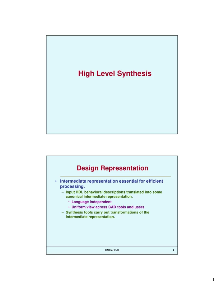
Design Representation
- Intermediate representation essential for efficient
processing.
– Input HDL behavioral descriptions translated into some canonical intermediate representation.
- Language independent
- Uniform view across CAD tools and users
– Synthesis tools carry out transformations of the intermediate representation.