
SLIDE 1
1
1
Hidden Markov Models (HMMs)
Raymond J. Mooney
University of Texas at Austin
2
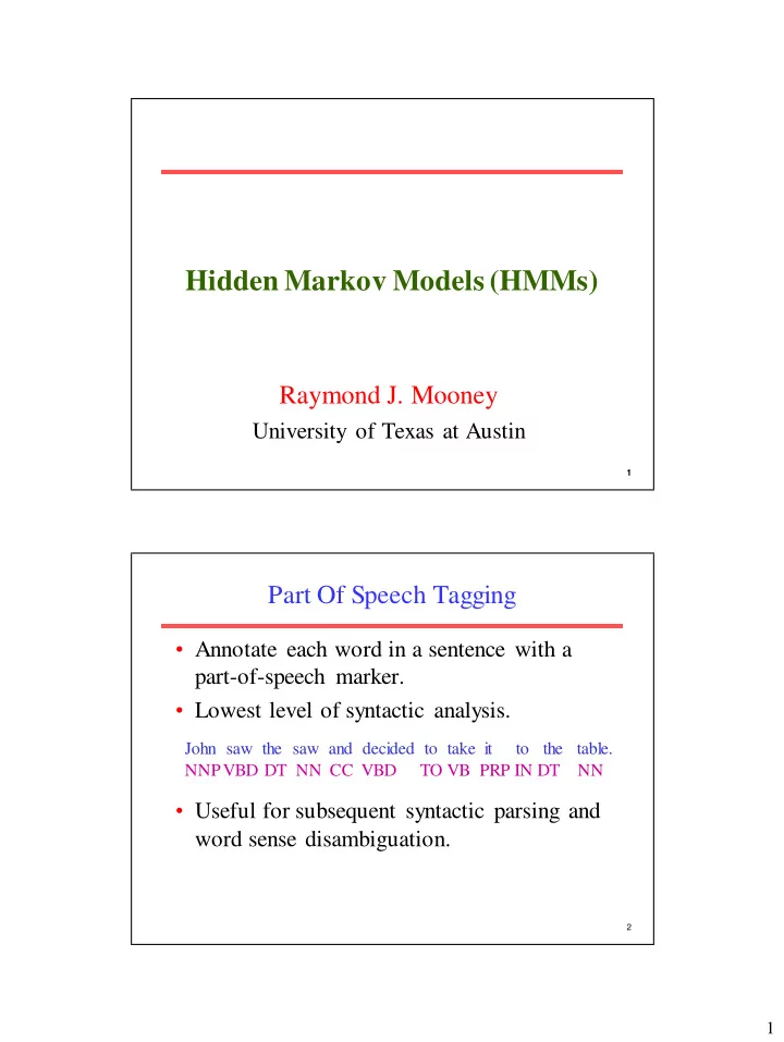
Part Of Speech Tagging
- Annotate each word in a sentence with a
part-of-speech marker.
- Lowest level of syntactic analysis.
- Useful for subsequent syntactic parsing and
word sense disambiguation.
John saw the saw and decided to take it to the table. NNP VBD DT NN CC VBD TO VB PRP IN DT NN