Hidden Markov Model (HMM) Sensor Markov assumption: P ( E t | X 0: t - - PDF document

hidden markov model hmm
SMART_READER_LITE
LIVE PREVIEW

Hidden Markov Model (HMM) Sensor Markov assumption: P ( E t | X 0: t - - PDF document

Hidden Markov Model (HMM) Sensor Markov assumption: P ( E t | X 0: t , E 1: t 1 ) = P ( E t | X t ) Stationary process: transition model P ( X t | X t 1 ) and Hidden Markov Models sensor model P ( E t | X t ) fixed for all t HMM is a


slide-1
SLIDE 1

Hidden Markov Models

AIMA Chapter 15, Sections 1–5

AIMA Chapter 15, Sections 1–5 1

Time and uncertainty

Consider a target tracking problem Xt = set of unobservable state variables at time t e.g., Positiont, Appearancet, etc. Et = set of observable evidence variables at time t e.g., Imagepixelst This assumes discrete time; step size depends on problem Notation: Xa:b = Xa, Xa+1, . . . , Xb−1, Xb

AIMA Chapter 15, Sections 1–5 2

Markov processes (Markov chains)

Construct a Bayes net from these variables: Markov assumption: Xt depends on bounded subset of X0:t−1 First-order Markov process: P(Xt|X0:t−1) = P(Xt|Xt−1) Second-order Markov process: P(Xt|X0:t−1) = P(Xt|Xt−2, Xt−1)

X t −1 X t X t −2 X t +1 X t +2 X t −1 X t X t −2 X t +1 X t +2

First−order Second−order

Stationary process: transition model P(Xt|Xt−1) fixed for all t

AIMA Chapter 15, Sections 1–5 3

Hidden Markov Model (HMM)

Sensor Markov assumption: P(Et|X0:t, E1:t−1) = P(Et|Xt) Stationary process: transition model P(Xt|Xt−1) and sensor model P(Et|Xt) fixed for all t HMM is a special type of Bayes net, Xt is single discrete random variable: with joint probability distribution P(X0:t, E1:t) = P(X0)Πt

i=1P(Xi|Xi−1)P(Ei|Xi)
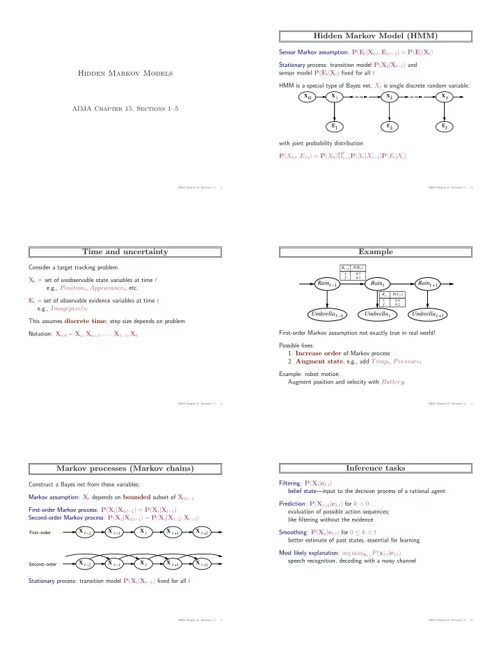
AIMA Chapter 15, Sections 1–5 4

Example

t

Rain

t

Umbrella Raint −1 Umbrellat −1 Raint +1 Umbrellat +1

Rt −1

t

P(R ) 0.3 f 0.7 t

t

R

t

P(U ) 0.9 t 0.2 f

First-order Markov assumption not exactly true in real world! Possible fixes:

  • 1. Increase order of Markov process
  • 2. Augment state, e.g., add Tempt, Pressuret

Example: robot motion. Augment position and velocity with Batteryt

AIMA Chapter 15, Sections 1–5 5

Inference tasks

Filtering: P(Xt|e1:t) belief state—input to the decision process of a rational agent Prediction: P(Xt+k|e1:t) for k > 0 evaluation of possible action sequences; like filtering without the evidence Smoothing: P(Xk|e1:t) for 0 ≤ k < t better estimate of past states, essential for learning Most likely explanation: arg maxx1:t P(x1:t|e1:t) speech recognition, decoding with a noisy channel

AIMA Chapter 15, Sections 1–5 6
slide-2
SLIDE 2

Filtering

Aim: devise a recursive state estimation algorithm: P(Xt+1|e1:t+1) = f(et+1, P(Xt|e1:t))

AIMA Chapter 15, Sections 1–5 7

Filtering

Aim: devise a recursive state estimation algorithm: P(Xt+1|e1:t+1) = f(et+1, P(Xt|e1:t)) P(Xt+1|e1:t+1) = P(Xt+1|e1:t, et+1) = αP(et+1|Xt+1, e1:t)P(Xt+1|e1:t) = αP(et+1|Xt+1)P(Xt+1|e1:t)

AIMA Chapter 15, Sections 1–5 8

Filtering

Aim: devise a recursive state estimation algorithm: P(Xt+1|e1:t+1) = f(et+1, P(Xt|e1:t)) P(Xt+1|e1:t+1) = P(Xt+1|e1:t, et+1) = αP(et+1|Xt+1, e1:t)P(Xt+1|e1:t) = αP(et+1|Xt+1)P(Xt+1|e1:t) I.e., prediction + estimation. Prediction by summing out Xt: P(Xt+1|e1:t+1) = αP(et+1|Xt+1)ΣxtP(Xt+1, xt|e1:t) = αP(et+1|Xt+1)ΣxtP(Xt+1|xt, e1:t)P(xt|e1:t) = αP(et+1|Xt+1)ΣxtP(Xt+1|xt)P(xt|e1:t)

AIMA Chapter 15, Sections 1–5 9

Filtering

Aim: devise a recursive state estimation algorithm: P(Xt+1|e1:t+1) = f(et+1, P(Xt|e1:t)) P(Xt+1|e1:t+1) = P(Xt+1|e1:t, et+1) = αP(et+1|Xt+1, e1:t)P(Xt+1|e1:t) = αP(et+1|Xt+1)P(Xt+1|e1:t) I.e., prediction + estimation. Prediction by summing out Xt: P(Xt+1|e1:t+1) = αP(et+1|Xt+1)ΣxtP(Xt+1, xt|e1:t) = αP(et+1|Xt+1)ΣxtP(Xt+1|xt, e1:t)P(xt|e1:t) = αP(et+1|Xt+1)ΣxtP(Xt+1|xt)P(xt|e1:t) f1:t+1 = Forward(f1:t, et+1) where f1:t = P(Xt|e1:t) Time and space constant (independent of t)

AIMA Chapter 15, Sections 1–5 10

Filtering example

Rain1 Umbrella1 Rain2 Umbrella2 Rain0

0.818 0.182 0.627 0.373 0.883 0.117 True False 0.500 0.500 0.500 0.500

P(Xt+1|e1:t+1) = αP(et+1|Xt+1)ΣxtP(Xt+1|xt)P(xt|e1:t)

Rt−1 P(Rt) t 0.7 f 0.3 Rt P(Ut) t 0.9 f 0.2

AIMA Chapter 15, Sections 1–5 11

Smoothing

X 0 X 1

1

E

t

E

t

X X k Ek

Divide evidence e1:t into e1:k, ek+1:t: P(Xk|e1:t) = P(Xk|e1:k, ek+1:t) = αP(Xk|e1:k)P(ek+1:t|Xk, e1:k) = αP(Xk|e1:k)P(ek+1:t|Xk) = αf1:kbk+1:t

AIMA Chapter 15, Sections 1–5 12
slide-3
SLIDE 3

Smoothing

X 0 X 1

1

E

t

E

t

X X k Ek

Divide evidence e1:t into e1:k, ek+1:t: P(Xk|e1:t) = P(Xk|e1:k, ek+1:t) = αP(Xk|e1:k)P(ek+1:t|Xk, e1:k) = αP(Xk|e1:k)P(ek+1:t|Xk) = αf1:kbk+1:t Backward message computed by a backwards recursion: P(ek+1:t|Xk) = Σxk+1P(ek+1:t|Xk, xk+1)P(xk+1|Xk) = Σxk+1P(ek+1:t|xk+1)P(xk+1|Xk) = Σxk+1P(ek+1|xk+1)P(ek+2:t|xk+1)P(xk+1|Xk)

AIMA Chapter 15, Sections 1–5 13

Smoothing example

Rain1 Umbrella1 Rain2 Umbrella2 Rain0

True False 0.818 0.182 0.627 0.373 0.883 0.117 0.500 0.500 0.500 0.500 1.000 1.000 0.690 0.410 0.883 0.117 forward backward smoothed 0.883 0.117

Forward–backward algorithm: cache forward messages along the way Time linear in t (polytree inference), space O(t|f|)

AIMA Chapter 15, Sections 1–5 14

Most likely explanation

AIMA Chapter 15, Sections 1–5 15

Most likely explanation

Most likely sequence = sequence of most likely states!!!! Most likely path to each xt+1 = most likely path to some xt plus one more step max

x1...xt P(x1, . . . , xt, Xt+1|e1:t+1)

= P(et+1|Xt+1) max

xt

 P(Xt+1|xt) max

x1...xt−1 P(x1, . . . , xt−1, xt|e1:t)

 

Identical to filtering, except f1:t replaced by m1:t = max

x1...xt−1 P(x1, . . . , xt−1, Xt|e1:t),

I.e., m1:t(i) gives the probability of the most likely path to state i. Update has sum replaced by max, giving the Viterbi algorithm: m1:t+1 = P(et+1|Xt+1) max

xt (P(Xt+1|xt)m1:t)

AIMA Chapter 15, Sections 1–5 16

Viterbi example

Rain1 Rain2 Rain3 Rain4 Rain5

true false true false true false true false true false .8182 .5155 .0361 .0334 .0210 .1818 .0491 .1237 .0173 .0024 m 1:1 m 1:5 m 1:4 m 1:3 m 1:2

state space paths most likely paths umbrella

true true true false true

AIMA Chapter 15, Sections 1–5 17

Example Umbrella Problems

Filtering: P(Xt+1|e1:t+1) = αP(et+1|Xt+1)ΣxtP(Xt+1|xt)P(xt|e1:t) =: f1:t+1 Smoothing: P(Xk|e1:t) = αf1:kbk+1:t P(ek+1:t|Xk) = Σxk+1P(ek+1|xk+1)P(ek+2:t|xk+1)P(xk+1|Xk) =: bk+1:t

Rt−1 P(Rt) t 0.7 f 0.3 Rt P(Ut) t 0.9 f 0.2

P(R3|¬u1, u2, ¬u3) = ? arg max

R1:3 P(R1:3|¬u1, u2, ¬u3) = ?

P(R2|¬u1, u2, ¬u3) = ?

AIMA Chapter 15, Sections 1–5 18