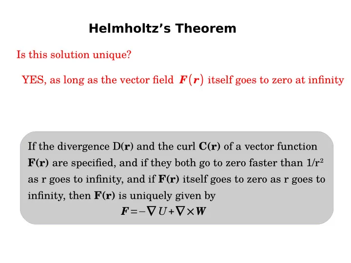
Helmholtzs Theorem I s t h i s s o l u t i o n u n i - PowerPoint PPT Presentation

Helmholtz’s Theorem I s t h i s s o l u t i o n u n i q u e ? Y E S , a s l o n g a s t h e v e c t o r f e l d ) i t s e l f g o e s t o z e r o a t i n f n i t t F ( r I f t h e d i v e r g e n c e D ( r ) a n d t h e c u r l C ( r ) o f a v e c t o r f u n c t i o n 2 F ( r ) a r e s p e c i f e d , a n d i f t h e t b o t h g o t o z e r o f a s t e r t h a n 1 / r a s r g o e s t o i n f n i t t , a n d i f F ( r ) i t s e l f g o e s t o z e r o a s r g o e s t o i n f n i t t , t h e n F ( r ) i s u n i q u e l t g i v e n b t F =−∇ U +∇ × W

Ma x w e l l ’ s E qu a t i on s E = ρ ∇ . ⃗ ϵ 0 ∇ . ⃗ B = 0 E =−∂ ⃗ B ∇× ⃗ ∂ t ∂ ⃗ E ∇× ⃗ B =μ 0 ⃗ J +μ 0 ϵ 0 ∂ t Maxwell’s equations specify the divergence and curl of the electric and magnetic fields. Using Helmholtz’s theorem, we can then determine the electric and magnetic fields from Maxwell’s equations.

Ma x w e l l ’ s E qu a t i on s - E L E C T R O O S S T A T I C S ∇ . E = ρ/ϵ 0 ∇ × E = 0 E ( r )=−∇ ( dV ' ) ρ( r ' ) 1 ℜ= r − r ' 4 πϵ 0 ∫ ℜ ρ( r ' ) 1 ^ 4 πϵ 0 ∫ = ℜ dV ' Coulomb’s Law! 2 ℜ σ( r ' ) 1 4 πϵ 0 ∫ ^ For a continuous surface charge, E ( r )= ℜ da' 2 ℜ λ( r ' ) 1 4 π ϵ 0 ∫ ^ For a continuous line charge, E ( r )= ℜ dl' 2 ℜ q i 1 2 ^ 4 π ϵ 0 ∑ For a collection of discrete charges, E ( r )= ℜ i ℜ i i

E L E C T R O S T A T I C S

E L E C T R O S T A T I C S ρ( r ' ) 1 4 πϵ 0 ∫ ^ E ( r )= ℜ dV ' 2 ℜ ∇ . E = ρ/ϵ 0 Helmholtz Theorem ∇ × E = 0 q i 1 4 πϵ 0 ∑ 2 ^ E ( r )= ℜ i ℜ i i Maxwell’s Equations for Electrostatics Coulomb’s Law Force on a test charge Q, F ( r )= Q E ( r ) z σ In principle, we’re done with Electrostatics!

E L E C T R i c F i e l d L i n e s ● Field lines begin on positive charges ● Field lines end on negative charges, or they extend upto infinity ● The strength of the field is indicated by the density of the field lines ● Field lines can never cross

E L E C T R i c F i e l d L i n e s – C l o o s s e d S u r f a c e Flux Φ E = ∮ S E . d S Flux ∝ Number of field lines Flux through a closed surface is a measure of the total charge inside the surface – Gauss’s Law

G a u s s ’ s L a w 4 π ϵ 0 ( r ) ( r q r )= q 1 ∮ E .d a = ∫ 2 ^ 2 sin θ d θ d ϕ ^ ϵ 0 r Point charge q at origin N E = ∑ Principle of superposition E i i = 1 ( ϵ 0 ) N N q i ∮ E .d a = ∑ ( ∮ E .d a ) = ∑ i = 1 i = 1 E .d a = 1 ∮ ϵ 0 Q enc Collection of point charges q i S

G a u s s ’ s L a w ^ q r .d S ∫ ∫ E .d S = 4 π ϵ 0 2 r surface surface | d S | cos θ q ∫ = 4 π ϵ 0 2 r surface d Ω= | d ⃗ S | cos θ q ∫ d Ω = = sin θ d θ d ϕ 4 π ϵ 0 2 r surface q q The solid angle subtended by a surface S is defined 4 π = = ϵ 0 as the surface area of a unit sphere covered by the 4 πϵ 0 surface's projection onto the sphere. A measure of how large an object appears to an observer looking from that point If the point is located outside then the contributions exactly cancel Use superposition principle ---> Add contribution from each charge

G a u s s ’ s L a w – D i f f e r e n t i a l F or m E .d S = ∫ ∫ ∇ . E dV surface vol ρ( r ) 1 ϵ 0 Q enc = ∫ ϵ 0 dV vol ϵ 0 Q enc ⇒ ∇ . E = ρ( r ) E .d a = 1 ∮ ϵ 0 S Helmholtz Theorem ∇ . E = ρ( r ) q 1 E = 2 ^ r ϵ 0 4 π ϵ 0 r Valid for moving charges! Only for static charges Gauss’s Law

C U R L OF T H E E L E C T R I C F I E L D q 1 2 ^ E = r 4 πϵ 0 r ∇ × E = 0 ( r ) . ( dr ^ b b 1 q E . d l = ∫ ∫ r + r d θ ^ θ+ r sin θ d ϕ ^ 2 ^ ϕ) b 4 πϵ 0 r a a 4 π ϵ 0 ( r b ) b b q q 1 1 − 1 ∫ 4 π ϵ 0 ∫ E . d l = 2 dr = r a r a a q ∮ E .d l = 0 ∇ × E = 0 Stokes Theorem ⇒ a True for any charge configuration due to superposition! Valid only for static charges

G a u s s ’ s L a w + S Y MME T R Y - S P H E R E Consider a spherically symmetric charge distribution ρ( r ) E ϕ = 0 Why? Rotate about the z-axis ∮ E . d l = 0 ⇒ E ϕ = 0 ρ( r ) E θ = 0 Why? Rotate about the x-axis ∮ E . d l = 0 ⇒ E θ = 0 R 2 = 1 ϵ 0 ∫ E r . 4 π R ρ( r ) 4 π r 2 .d r Apply Gauss's Law: 0

G a u s s ’ s L a w + S Y MME T R Y - C Y L I N D E R Consider a long, narrow wire with a charge per unit length λ E ϕ = 0 Why? Rotate about the z-axis ∮ E . d l = 0 ⇒ E ϕ = 0 E z = 0 Why? Flip about z-axis Nothing distinguishes z from -z ⇒ E z = 0 E ρ . 2 πρ = 1 ϵ 0 λ Apply Gauss's Law:

G a u s s ’ s L a w + S Y MME T R Y - S U R F A C E Consider an infinite sheet of charge with a surface charge density σ E // ( E x , E y )= 0 Why? Rotate the sheet about any point Translate by any in-plane vector ⇒ E // = 0 Field cannot change ∫ E .d a = 2 A | E | = 1 ϵ 0 σ A Apply Gauss's Law: E = σ ^ n 2 ϵ 0

G a u s s ’ s L a w + S Y MME T R Y - S U R F A C E Consider two parallel plates with equal and opposite charge densities ±σ . What is the electric field? ϵ 0 A C = d σ −σ E = { σ n + σ n = σ ^ ^ ϵ 0 ^ n between the plates 2 ϵ 0 2 ϵ 0 0 everywhere else

G a u s s ’ s L a w + S y mme t r y What is the flux of the electric field through the shaded face? q 24 ϵ 0

T H E E L E C T R I C P O T E N T I A L Gauss’s Law is always true. It may not always be useful! If we can take advantage of the symmetries of a problem, Gauss’s Law can be a very powerful tool. ∇ × E = 0 E = −∇ V V ( r ) ≡ Electric Potential Poisson’s Equation 2 V =−ρ/ϵ 0 ∇ . E =ρ/ϵ 0 ⇒ ∇ In regions of no charge ∇ 2 V = 0 Laplace Equation