Hashing CptS 223 Advanced Data Structures Larry Holder School of - PowerPoint PPT Presentation
Hashing CptS 223 Advanced Data Structures Larry Holder School of Electrical Engineering and Computer Science Washington State University 1 Overview Hashing Technique supporting insertion, deletion and search in average-case
Hashing CptS 223 – Advanced Data Structures Larry Holder School of Electrical Engineering and Computer Science Washington State University 1
Overview � Hashing � Technique supporting insertion, deletion and search in average-case constant time � Operations requiring elements to be sorted (e.g., FindMin) are not efficiently supported � Hash table ADT � Implementations � Analysis � Applications 2
Hash Table � One approach � Hash table is an array of fixed size TableSize � Array elements indexed by a key, which is mapped to an array index (0…TableSize-1) � Mapping (hash function) h from key to index � E.g., h(“john”) = 3 3
Hash Table � Insert � T [h(“john”] = <“john”,25000> � Delete � T [h(“john”)] = NULL � Search � Return T [h(“john”)] � What if h(“john”) = h(“joe”) ? 4
Hash Function � Mapping from key to array index is called a hash function � Typically, many-to-one mapping � Different keys map to different indices � Distributes keys evenly over table � Collision occurs when hash function maps two keys to same array index 5
Hash Function � Simple hash function � h(Key) = Key mod TableSize � Assumes integer keys � For random keys, h() distributes keys evenly over table � What if TableSize = 100 and keys are multiples of 10? � Better if TableSize is a prime number � Not too close to powers of 2 or 10 6
Hash Function for String Keys � Approach 1 � Add up character ASCII values (0-127) to produce integer keys � Small strings may not use all of table � Strlen(S) * 127 < TableSize � Approach 2 � Treat first 3 characters of string as base-27 integer (26 letters plus space) � Key = S[0] + (27 * S[1]) + (27 2 * S[2]) � Assumes first 3 characters randomly distributed � Not true of English 7
Hash Function for String Keys Approach 3 � Use all N characters of string as � an N-digit base-K integer Choose K to be prime number � larger than number of different digits (characters) I.e., K = 29, 31, 37 � If L = length of string S, then � ⎡ ⎤ − = ∑ L 1 i mod − − ∗ h ( S ) S [ L i 1 ] 37 TableSize ⎢ ⎥ ⎣ ⎦ = i 0 Use Horner’s rule to compute h(S) � Limit L for long strings � 8
Collision Resolution � What happens when h(k 1 ) = h(k 2 )? � Collision resolution strategies � Chaining � Store colliding keys in a linked list � Open addressing � Store colliding keys elsewhere in the table 9
Collision Resolution by Chaining � Hash table T is a vector of lists � Only singly-linked lists needed if memory is tight � Key k is stored in list at T[h(k)] � E.g., TableSize = 10 � h(k) = k mod 10 � Insert first 10 perfect squares 10
Implementation of Chaining Hash Table Generic hash functions for integers and keys 11
Implementation of Chaining Hash Table 12
STL algorithm: find Each of these operations takes time linear in the length of the list. 13
No duplicates Later, but essentially doubles size of table and reinserts current elements. 14
All hash objects must define == and != operators. Hash function to handle Employee object type 15
Collision Resolution by Chaining: Analysis � Load factor λ of a hash table T � N = number of elements in T � M = size of T � λ = N/M � Average length of a chain is λ � Unsuccessful search O( λ ) � Successful search O( λ /2) � Ideally, want λ ≈ 1 (not a function of N) � I.e., TableSize = number of elements you expect to store in the table 16
Collision Resolution by Open Addressing � When a collision occurs, look elsewhere in the table for an empty slot � Advantages over chaining � No need for addition list structures � No need to allocate/deallocate memory during insertion/deletion (slow) � Disadvantages � Slower insertion – May need several attempts to find an empty slot � Table needs to be bigger (than chaining-based table) to achieve average-case constant-time performance � Load factor λ ≈ 0.5 17
Collision Resolution by Open Addressing � Probe sequence � Sequence of slots in hash table to search � h 0 (x), h 1 (x), h 2 (x), … � Needs to visit each slot exactly once � Needs to be repeatable (so we can find/delete what we’ve inserted) � Hash function � h i (x) = (h(x) + f(i)) mod TableSize � f(0) = 0 18
Linear Probing � f(i) is a linear function of i � E.g., f(i) = i � Example: h(x) = x mod TableSize � h 0 (89) = (h(89)+f(0)) mod 10 = 9 � h 0 (18) = (h(18)+f(0)) mod 10 = 8 � h 0 (49) = (h(49)+f(0)) mod 10 = 9 (X) � h 1 (49) = (h(49)+f(1)) mod 10 = 0 19
Linear Probing Example 20
Linear Probing: Analysis � Probe sequences can get long � Primary clustering � Keys tend to cluster in one part of table � Keys that hash into cluster will be added to the end of the cluster (making it even bigger) 21
Linear Probing: Analysis � Expected number of � Example ( λ = 0.5) probes for insertion or � Insert / unsuccessful unsuccessful search search � 2.5 probes ⎛ ⎞ 1 1 ⎜ ⎟ + 1 � Successful search ⎜ ⎟ − λ 2 ⎝ ⎠ 2 ( 1 ) � 1.5 probes � Expected number of � Example ( λ = 0.9) probes for successful � Insert / unsuccessful search search ⎛ ⎞ � 50.5 probes 1 1 ⎜ + ⎟ 1 ⎜ ⎟ � Successful search − λ ⎝ ⎠ 2 ( 1 ) � 5.5 probes 22
Random Probing: Analysis � Random probing does not suffer from clustering � Expected number of probes for insertion or unsuccessful search: 1 1 ln λ − λ 1 � Example � λ = 0.5: 1.4 probes � λ = 0.9: 2.6 probes 23
Linear vs. Random Probing # probes Linear probing Random probing Load factor λ 24
Quadratic Probing � Avoids primary clustering � f(i) is quadratic in i � E.g., f(i) = i 2 � Example � h 0 (58) = (h(58)+f(0)) mod 10 = 8 (X) � h 1 (58) = (h(58)+f(1)) mod 10 = 9 (X) � h 2 (58) = (h(58)+f(2)) mod 10 = 2 25
Quadratic Probing Example 26
Quadratic Probing: Analysis � Difficult to analyze � Theorem 5.1 � New element can always be inserted into a table that is at least half empty and TableSize is prime � Otherwise, may never find an empty slot, even is one exists � Ensure table never gets half full � If close, then expand it 27
Quadratic Probing � Only M (TableSize) different probe sequences � May cause “secondary clustering” � Deletion � Emptying slots can break probe sequence � Lazy deletion � Differentiate between empty and deleted slot � Skip deleted slots � Slows operations (effectively increases λ ) 28
Quadratic Probing: Implementation 29
Quadratic Probing: Implementation Lazy deletion 30
Quadratic Probing: Implementation Ensure table size is prime 31
Quadratic Probing: Implementation Find Skip DELETED; No duplicates Quadratic probe sequence (really) 32
Quadratic Probing: Implementation Insert No duplicates Remove No deallocation needed 33
Double Hashing � Combine two different hash functions � f(i) = i * h 2 (x) � Good choices for h 2 (x) ? � Should never evaluate to 0 � h 2 (x) = R – (x mod R) � R is prime number less than TableSize � Previous example with R=7 � h 0 (49) = (h(49)+f(0)) mod 10 = 9 (X) � h 1 (49) = (h(49)+(7 – 49 mod 7)) mod 10 = 6 34
Double Hashing Example 35
Double Hashing: Analysis � Imperative that TableSize is prime � E.g., insert 23 into previous table � Empirical tests show double hashing close to random hashing � Extra hash function takes extra time to compute 36
Rehashing � Increase the size of the hash table when load factor too high � Typically expand the table to twice its size (but still prime) � Reinsert existing elements into new hash table 37
Rehashing Example h(x) = x mod 7 h(x) = x mod 17 λ = 0.57 λ = 0.29 Rehashing Insert 23 λ = 0.71 38
Rehashing Analysis � Rehashing takes O(N) time � But happens infrequently � Specifically � Must have been N/2 insertions since last rehash � Amortizing the O(N) cost over the N/2 prior insertions yields only constant additional time per insertion 39
Rehashing Implementation � When to rehash � When table is half full ( λ = 0.5) � When an insertion fails � When load factor reaches some threshold � Works for chaining and open addressing 40
Rehashing for Chaining 41
Rehashing for Quadratic Probing 42
Hash Tables in C++ STL � Hash tables not part of the C++ Standard Library � Some implementations of STL have hash tables (e.g., SGI’s STL) � hash_set � hash_map 43
Recommend
More recommend
Explore More Topics
Stay informed with curated content and fresh updates.


![Union-Find [10] In the last class Hashing Collision Handling for Hashing Closed](https://c.sambuz.com/1022731/union-find-s.webp)
