Half Toning Color Half Toning 1 Color Half Toning 2 Half Toning - - PDF document

half toning color half toning
SMART_READER_LITE
LIVE PREVIEW

Half Toning Color Half Toning 1 Color Half Toning 2 Half Toning - - PDF document

Half Toning Color Half Toning 1 Color Half Toning 2 Half Toning Emulating 5 different levels (0) (1) (2) (3) (4) (0) (1) (2) (3) (0) (1) (2) (3) (4) Half Toning (2) (0) (1) (3) (4) (7) (5) (6) (8) (9) 10 levels 3 4


slide-1
SLIDE 1

1

Half Toning Color Half Toning

slide-2
SLIDE 2

2

Color Half Toning

slide-3
SLIDE 3

3

(0) (1) (2) (3) (4) (0) (1) (2) (3) (0) (1) (2) (3) (4)

Emulating 5 different levels

Half Toning

(0) (1) (2) (3) (4) (5) (6) (7) (8) (9)

Half Toning

10 levels

slide-4
SLIDE 4

4

slide-5
SLIDE 5

5

Dithering and Halftoning

Trade spatial for intensity resolution (works well for printing where dot printing is very high)

  • Thresholding.
  • Random dither; Robert’s algorithm
  • Ordered dither
  • Error diffusion

Your eye will average over an area

  • Spatial Integration
slide-6
SLIDE 6

6

Thresholding

Assume we want to quantize a gray-level image to a binary colormap. Map the upper half of the gray-level scale to white, and the lower half to black – a simple threshold operation, preformed independently at each pixel.

Thresholding.

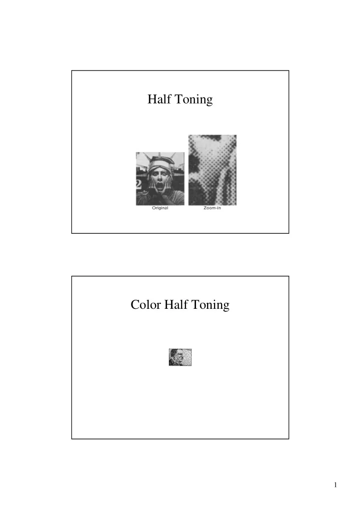
Original image. Simple threshold.

n = 0.5 n= 0.7

) ) , ( ( ) , ( n y x v trunc y x v

  • Errors are low spatial frequencies.
slide-7
SLIDE 7

7

Robert’s Algorithm

  • First add noise
  • Then quantize

x i

1

r r + 1

Quantised to 1 Quantised to 0

)) , ( ) , ( ( ) , ( y x noise y x v K trunc y x v

  • 1
  • noise

Moves errors to higher spatial frequencies.

  • > eye averages over an area.

Robert’s Algorithm

Moves low frequency (average error) to high frequency Pink(low), Blue (high), White(all) frequency noise

Pink Blue

slide-8
SLIDE 8

8

The trouble with noise.

  • Difficult to compute quickly.
  • Not reproducible.
  • Pre-compute pseudo-random function and

store in table.

  • Small tiled patterns sufficient
slide-9
SLIDE 9

9

Each pixel produces a quatization error The quality of the result may be improved by adjusting the threshold locally, so that adjacent pixels in small areas are quantized with different thresholds. This reduces the average local quantization

  • error. Matrices of these threshold are called

dither matrices.

Dithering Comparison

slide-10
SLIDE 10

10

Ordered Dithering

  • Trade off spatial

resolution for intensity resolution.

  • Use dither patterns.
  • Can be represented as

a matrix.

Bayer Ordered Dither Patterns

slide-11
SLIDE 11

11

Other possibilities.

9 4 8 6 1 2 5 7 3

For all Xpixels For all Ypixels v = approximate(x,y) i = x mod m j = y mod n if v >= M[i,j] then Set_Pixel(x,y, BLACK) else Set_Pixel(x,y, WHITE) The dithering matrix (3x3)

slide-12
SLIDE 12

12

Dithering

9 4 8 6 1 2 5 7 3 9 4 8 6 1 2 5 7 3 9 4 8 6 1 2 5 7 3 9 4 8 6 1 2 5 7 3 9 4 8 6 1 5 7 3 2 5 5 4 4 4 2 2 2 2 2 3 3 3 3 6 8 4 4 4 4 2 2 8 3 8 8 9 9 9 8 8 7 7 7 7 6 4 2 4 4 2 2 1 2 2 2 3 3 8 4 4 9 4 8 6 1 2 5 7 3 1 1 1 1 1

Dithering mask Image Binary image

Comparison.

slide-13
SLIDE 13

13

Floyd-Steinberg Error Diffusion

With this method, the average quatization error is reduced by propagating the error from each pixel to some of its neighbors in the scan order. Note that the error propagation weights must sum to one e

  • 3e/8
  • 3e/8
  • e/4

Dither vs. Floyd-Steinberg

slide-14
SLIDE 14

14

Set AccErr[] to zero; For each pixel in the image scanning from left to right: value= Pixel_value(x,y) + AccErr[x,y]; if (value > WHITE/2) { Set_pixel(x,y, WHITE); Error = value - WHITE; } else { Set_pixel(x,y, BLACK); Error = value - BLACK; } if scanning from left to right { AccErr[x+1, y] += 3/8 * Error; AccErr[x, y+1] += 3/8 * Error; AccErr[x+1,y+1] += 2/8 * Error; }

Error Diffusion

slide-15
SLIDE 15

15

slide-16
SLIDE 16

16

Median Cut

slide-17
SLIDE 17

17

Median Cut Median Cut

slide-18
SLIDE 18

18

Median Cut Median Cut

slide-19
SLIDE 19

19

Median Cut

slide-20
SLIDE 20

20

A better solution

slide-21
SLIDE 21

21

Median Cut

Original image 8 indexed colored

slide-22
SLIDE 22

22 8 indexed colored 32 indexed colored 128 indexed colored Original image

slide-23
SLIDE 23

23 8 levels per channel that is, 9 bits per pixel