h [.,.] h [.,.] f [.,.] f [.,.] 0 0 0 0 0 0 0 0 0 0 - - PowerPoint PPT Presentation

BBM 413 Fundamentals of Image Processing

Erkut Erdem

• Dept. of Computer Engineering

Hacettepe University

Frequency Domain Techniques – Part1

Review - Point Operations

• Smallest possible neighborhood is of size 1x1
• Process each point independently of the others
• Output image g depends only on the value of f

at a single point (x,y)

• Transformation function T remaps the sample’s value:

s = T(r) where

– r is the value at the point in question – s is the new value in the processed result – T is a intensity transformation function

90 90 90 90 90 90 90 90 90 90 90 90 90 90 90 90 90 90 90 90 90 90 90 90 90 90 90 90 90 90 90 90 90 90 90 90 90 90 90 90 90 90 90 90 90 90 90 90 90 90

] , [ ] , [ ] , [

,

l n k m f l k g n m h

l k

+ + =å

[.,.] h [.,.] f

1 1 1 1 1 1 1 1 1

] , [ g × ×

Slide credit: S. Seitz

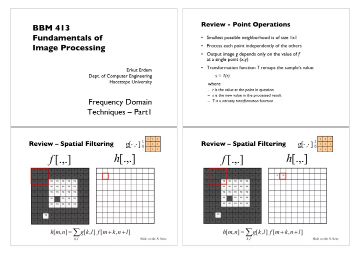
Review – Spatial Filtering

90 90 90 90 90 90 90 90 90 90 90 90 90 90 90 90 90 90 90 90 90 90 90 90 90 10 90 90 90 90 90 90 90 90 90 90 90 90 90 90 90 90 90 90 90 90 90 90 90 90 90

[.,.] h [.,.] f

1 1 1 1 1 1 1 1 1

] , [ g × ×

] , [ ] , [ ] , [

,

l n k m f l k g n m h

l k

+ + =å

Slide credit: S. Seitz

Review – Spatial Filtering

90 90 90 90 90 90 90 90 90 90 90 90 90 90 90 90 90 90 90 90 90 90 90 90 90 10 20 90 90 90 90 90 90 90 90 90 90 90 90 90 90 90 90 90 90 90 90 90 90 90 90 90

[.,.] h [.,.] f

1 1 1 1 1 1 1 1 1

] , [ g × ×

] , [ ] , [ ] , [

,

l n k m f l k g n m h

l k

+ + =å

Slide credit: S. Seitz

Review – Spatial Filtering

90 90 90 90 90 90 90 90 90 90 90 90 90 90 90 90 90 90 90 90 90 90 90 90 90 10 20 30 90 90 90 90 90 90 90 90 90 90 90 90 90 90 90 90 90 90 90 90 90 90 90 90 90

[.,.] h [.,.] f

1 1 1 1 1 1 1 1 1

] , [ g × ×

] , [ ] , [ ] , [

,

l n k m f l k g n m h

l k

+ + =å

Slide credit: S. Seitz

Review – Spatial Filtering

10 20 30 30 90 90 90 90 90 90 90 90 90 90 90 90 90 90 90 90 90 90 90 90 90 90 90 90 90

[.,.] h [.,.] f

1 1 1 1 1 1 1 1 1

] , [ g × ×

] , [ ] , [ ] , [

,

l n k m f l k g n m h

l k

+ + =å

Slide credit: S. Seitz

Review – Spatial Filtering

90 90 90 90 90 90 90 90 90 90 90 90 90 90 90 90 90 90 90 90 90 90 90 90 90 10 20 30 30 30 20 10 20 40 60 60 60 40 20 30 60 90 90 90 60 30 30 50 80 80 90 60 30 30 50 80 80 90 60 30 20 30 50 50 60 40 20 10 20 30 30 30 30 20 10 10 10 10

[.,.] h [.,.] f

] , [ ] , [ ] , [

,

l n k m f l k g n m h

l k

+ + =å

1 1 1 1 1 1 1 1 1

] , [ g × ×

Slide credit: S. Seitz

Review – Spatial Filtering

• 1

1

• 2

2

• 1

1

Sobel

Slide credit: J. Hays

Review – Spatial Filtering Review – Spatial Filtering

Fill in the blanks: a) _ = D * B b) A = _ * _ c) F = D * _ d) _ = D * D A B C D E F G H I

Filtering Operator

Slide credit: D. Hoiem

Today

• Frequency domain techniques
• Images in terms of frequency
• Fourier Series
• Convolution Theorem

Why does the Gaussian give a nice smooth image, but the square filter give edgy artifacts? Gaussian Box filter

Slide credit: D. Hoiem

Why does a lower resolution image still make sense to us? What do we lose?

Image: http://www.flickr.com/photos/igorms/136916757/

Slide credit: D. Hoiem

How is it that a 4MP image can be compressed to a few hundred KB without a noticeable change?

Slide credit: J. Hays

Answer to these questions?

• Thinking images in terms of frequency.
• Treat images as infinite-size, continuous periodic

functions.

=&

)&

=& ...& ...& ...& ...&

Jean Baptiste Joseph Fourier (1768-1830) had crazy idea (1807):

Any univariate function can be rewritten as a weighted sum of sines and cosines of different frequencies.

Slide credit: A. Efros

Jean Baptiste Joseph Fourier (1768-1830) had crazy idea (1807):

Any univariate function can be rewritten as a weighted sum of sines and cosines of different frequencies.

• Don’t believe it?

– Neither did Lagrange, Laplace, Poisson and

• ther big wigs

– Not translated into English until 1878! ...the manner in which the author arrives at these equations is not exempt of difficulties and...his analysis to integrate them still leaves something to be desired

• n the score of generality and even rigour.

Laplace Lagrange Legendre

Jean Baptiste Joseph Fourier (1768-1830) had crazy idea (1807):

Any univariate function can be rewritten as a weighted sum of sines and cosines of different frequencies.

• Don’t believe it?

– Neither did Lagrange, Laplace, Poisson and

• ther big wigs

– Not translated into English until 1878!

• But it’s (mostly) true!

– called Fourier Series – there are some subtle restrictions

Slide credit: A. Efros

A sum of sines

Our building block: Add enough of them to get any signal f(x) you want!

) +f wx Asin(

Slide credit: A. Efros

Frequency Spectra

• example: g(t) = sin(2πf t) + (1/3)sin(2π(3f) t)

= +

Slide credit: A. Efros

Frequency Spectra

Slide credit: A. Efros

= + =

Frequency Spectra

Slide credit: A. Efros

= + =

Frequency Spectra

Slide credit: A. Efros

= + =

Frequency Spectra

Slide credit: A. Efros

= + =

Frequency Spectra

Slide credit: A. Efros

= + =

Frequency Spectra

Slide credit: A. Efros

=

1

1 sin(2 )

k

A kt k p

¥ =

å

Frequency Spectra

Slide credit: A. Efros

Frequency Spectra

Image credit: Lucas V. Barbosa

Example: Music

• We think of music in terms of frequencies at different

magnitudes.

Slide credit: D . Hoeim

Other signals

• We can also think of all kinds of other signals the same way

xkcd.com

Slide credit: J. Hays

Fourier Transform

We want to understand the frequency w of our signal. So, let’s reparametrize the signal by w instead of x:

) +f wx Asin(

f( f(x) F( F(w)

Fourier Transform

F( F(w) f( f(x)

Inverse Fourier Transform For every w from 0 to inf, F(w) holds the amplitude A and phase f of the corresponding sine

• How can F hold both? Complex number trick!

) ( ) ( ) ( w w w iI R F + =

2 2

) ( ) ( w w I R A + ± = ) ( ) ( tan 1 w w f R I

• =

We can always go back:

Slide credit: A. Efros

• Fourier transform stores the magnitude and phase at each

frequency

– Magnitude encodes how much signal there is at a particular frequency – Phase encodes spatial information (indirectly) – For mathematical convenience, this is often notated in terms of real and complex numbers

2 2

) ( ) ( w w I R A + ± = ) ( ) ( tan 1 w w f R I

• =

Amplitude: Phase:

Fourier Transform

Slide credit: B. Freeman and A. Torralba

Discrete Fourier transform

• Forward transform
• Inverse transform

Euler’s definition of eiθ

u, v : the transform or frequency variables x, y : the spatial or image variables

F(u,v) = 1 MN f (x, y)e− j2π (ux/M+vy/N )

y=0 N−1

∑

x=0 M−1

∑

for u = 0,1,2,..., M −1,v = 0,1,2,..., N −1

1 ,..., 2 , 1 , , 1 ,..., 2 , 1 , for ) , ( ) , (

1 1 ) / / ( 2

• =
• =

= åå

• =
• =

+

N y M x e v u F y x f

M u N v N vy M ux j p

The Fourier Transform

• Represent function on a new basis

– Think of functions as vectors, with many components – We now apply a linear transformation to transform the basis

• dot product with each basis element
• In the expression, u and v select the basis

element, so a function of x and y becomes a function of u and v

• basis elements have the form e−i2π ux+vy

( )

Slide credit: S. Thrun

Horizontal

• rientation

Vertical orientation

45 deg.

fmax

fx in cycles/image Low spatial frequencies High spatial frequencies

Slide credit: B. Freeman and A. Torralba

How to interpret 2D Fourier Spectrum

Log power spectrum

Fourier basis element example, real part Fu,v(x,y) Fu,v(x,y)=const. for (ux+vy)=const. Vector (u,v)

• Magnitude gives frequency
• Direction gives orientation.

e−i2π ux+vy

( ) Slide credit: S. Thrun

Here u and v are larger than in the previous slide.

Slide credit: S. Thrun

And larger still...

Slide credit: S. Thrun

2D FFT

Sinusoid with frequency = 1 and its FFT

Slide credit: M. H. Yang

2D FFT

Sinusoid with frequency = 3 and its FFT

Slide credit: M. H. Yang

2D FFT

Sinusoid with frequency = 5 and its FFT

Slide credit: M. H. Yang

2D FFT

Sinusoid with frequency = 10 and its FFT

Slide credit: M. H. Yang

2D FFT

Sinusoid with frequency = 15 and its FFT

Slide credit: M. H. Yang

2D FFT

Sinusoid with varying frequency and their FFT

Slide credit: M. H. Yang

Rotation

Sinusoid rotated at 30 degrees and its FFT

Slide credit: M. H. Yang

2D FFT

Sinusoid rotated at 60 degrees and its FFT

Slide credit: M. H. Yang

2D FFT

Slide credit: M. H. Yang

Fourier analysis in images

Intensity Image Fourier Image

http://sharp.bu.edu/~slehar/fourier/fourier.html#filtering More: http://www.cs.unm.edu/~brayer/vision/fourier.html

Slide credit: A. Efros

Signals can be composed + =

http://sharp.bu.edu/~slehar/fourier/fourier.html#filtering More: http://www.cs.unm.edu/~brayer/vision/fourier.html

Slide credit: A. Efros

Some important Fourier Transforms

Image Magnitude FT

Slide credit: B. Freeman and A. Torralba

Some important Fourier Transforms

Image Magnitude FT

Slide credit: B. Freeman and A. Torralba

The Fourier Transform of some important images

Image Log(1+Magnitude FT)

Slide credit: B. Freeman and A. Torralba

The Fourier Transform of some well-known images

A B C 1 2 3

fx(cycles/image pixel size) fx(cycles/image pixel size) fx(cycles/image pixel size)

Slide credit: B. Freeman and A. Torralba

Fourier Amplitude Spectrum Fourier transform magnitude

Slide credit: B. Freeman and A. Torralba

What in the image causes the dots?

Masking out the fundamental and harmonics from periodic pillars

Slide credit: B. Freeman and A. Torralba

The Convolution Theorem

• The Fourier transform of the convolution of two

functions is the product of their Fourier transforms

• The inverse Fourier transform of the product of two

Fourier transforms is the convolution of the two inverse Fourier transforms

• Convolution in spatial domain is equivalent to

multiplication in frequency domain!

] F[ ] F[ ] F[ h g h g = *

] [ F ] [ F ] [ F

1 1 1

h g gh

• *

=

Slide credit: A. Efros

Properties of Fourier Transforms

• Linearity
• Fourier transform of a real signal is symmetric about

the origin

• The energy of the signal is the same as the energy of

its Fourier transform

Slide credit: J. Hays

Filtering in spatial domain

• 1

1

• 2

2

• 1

1

*

=

Slide credit: D. Hoiem

Filtering in frequency domain

FFT FFT Inverse FFT

=

Slide credit: D. Hoiem

2D convolution theorem example

* f(x,y) h(x,y) g(x,y) |F(sx,sy)| |H(sx,sy)| |G(sx,sy)|

Slide credit: A. Efros

Why does the Gaussian give a nice smooth image, but the square filter give edgy artifacts?

Gaussian Box filter

Filtering

Slide credit: A. Efros

Gaussian

Slide credit: A. Efros

Filtering

Box Filter

Slide credit: A. Efros

Filtering Fourier Transform pairs

Slide credit: A. Efros

Low-pass, Band-pass, High-pass filters

low-pass: High-pass / band-pass:

Slide credit: A. Efros

Edges in images

Slide credit: A. Efros

FFT in Matlab

• Filtering with fft
• Displaying with fft

im = ... % “im” should be a gray-scale floating point image [imh, imw] = size(im); fftsize = 1024; % should be order of 2 (for speed) and include padding im_fft = fft2(im, fftsize, fftsize); % 1) fft im with padding hs = 50; % filter half-size fil = fspecial('gaussian', hs*2+1, 10); fil_fft = fft2(fil, fftsize, fftsize); % 2) fft fil, pad to same size as image im_fil_fft = im_fft .* fil_fft; % 3) multiply fft images im_fil = ifft2(im_fil_fft); % 4) inverse fft2 im_fil = im_fil(1+hs:size(im,1)+hs, 1+hs:size(im, 2)+hs); % 5) remove padding figure(1), imagesc(log(abs(fftshift(im_fft)))), axis image, colormap jet Slide credit: D. Hoiem

Phase and Magnitude

• Curious fact

– all natural images have about the same magnitude transform – hence, phase seems to matter, but magnitude largely doesn’t

• Demonstration

– Take two pictures, swap the phase transforms, compute the inverse - what does the result look like?

Image with zebra phase

th

(and cheetah magnitude) Slide credit: B. Freeman and A. Torralba Image with cheetah phase (and zebra magnitude) Image with zebra phase (and cheetah magnitude)

Slide credit: B. Freeman and A. Torralba

This is the magnitude transform of the cheetah picture

Slide credit: B. Freeman and A. Torralba Slide credit: B. Freeman and A. Torralba

This is the magnitude transform of the zebra picture

Slide credit: B. Freeman and A. Torralba

Reconstruction with zebra phase, cheetah magnitude

Slide credit: B. Freeman and A. Torralba

Reconstruction with cheetah phase, zebra magnitude

Slide credit: B. Freeman and A. Torralba

• Early processing in humans filters for various orientations and scales of

frequency

• Perceptual cues in the mid-high frequencies dominate perception
• When we see an image from far away, we are effectively subsampling it

Early Visual Processing: Multi-scale edge and blob filters

Clues from Human Perception

Slide credit: J. Hays

Campbell-Robson contrast sensitivity curve

The higher the frequency the less sensitiv The higher the frequency the less sensitive human visual system is...

Slide credit: J. Hays

Lossy Image Compression (JPEG)

Block-based Discrete Cosine Transform (DCT) on 8x8 Slide credit: A. Bobick

Using DCT in JPEG

• The first coefficient B(0,0) is the DC component, the average

intensity

• The top-left coeffs represent low frequencies,

the bottom right – high frequencies

Slide credit: A. Bobick

Image compression using DCT

• DCT enables image compression by concentrating most image

information in the low frequencies

• Loose unimportant image info (high frequencies) by cutting

B(u,v) at bottom right

• The decoder computes the inverse DCT – IDCT

Slide credit: A. Bobick

JPEG compression comparison

89k 12k

Slide credit: A. Bobick

Things to Remember

• Sometimes it makes sense to think of images

and filtering in the frequency domain

– Fourier analysis

• Can be faster to filter using FFT for large

images (N logN vs. N2 for auto-correlation)

• Images are mostly smooth

– Basis for compression

Slide credit: J. Hays

Practice question

1. Match the spatial domain image to the Fourier magnitude image 1 5 4 A 3 2 C B D E

Slide credit: J. Hays

Summary

• Frequency domain techniques
• Images in terms of frequency
• Fourier Series
• Convolution Theorem

Next Week

• Sampling
• Gabor wavelets
• Steerable filters