Growth and Shared Prosperity in Brazil Marcelo Neri FGV Social and - - PDF document

20/03/2019 1

Growth and Shared Prosperity in Brazil

Marcelo Neri FGV Social and EPGE/FGV With Nanak Kakwani and Fabio Vaz References: * 9 these slides

http://www.cps.fgv.br/cps/bd/curso/9-Slides-Growth-and-shared-prosperity-in-Brasil.pdf

** 10 Paper

http://www.cps.fgv.br/cps/bd/curso/10-Growth-and-Shared-Prosperity-in-Brazil.pdf

** Video Paper Presentation Short 4 min (Port)

http://cps.fgv.br/videos/anpec-growth-and-shared-prosperity-brazil-0353

****Video Paper Presentation Long 24 min (Port)

http://cps.fgv.br/videos/anpec-growth-and-shared-prosperity-brazil-integra-2410

1

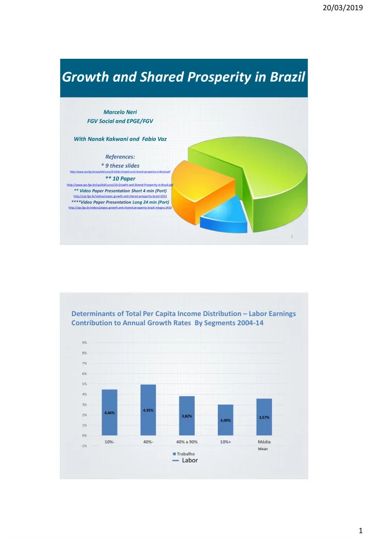
Determinants of Total Per Capita Income Distribution – Labor Earnings Contribution to Annual Growth Rates By Segments 2004-14

4,46% 4,95% 3,82% 3,00% 3,57%

• 1%

0% 1% 2% 3% 4% 5% 6% 7% 8% 9%

10%- 40%- 40% a 90% 10%+ Média Trabalho

Mean

Labor

20/03/2019 2

Determinants of Total Per Capita Income Distribution – By Income Sources Contribution to Annual Growth Rates By Segments 2004-14

4,46% 4,95% 3,82% 3,00% 3,57% 0,72% 0,89% 0,49% 0,03% 0,32% 0,06% 0,28% 0,66% 0,50% 0,57% 2,47% 0,80% 0,11%

• 0,02%

0,14%

• 1%

0% 1% 2% 3% 4% 5% 6% 7% 8% 9% 10%- 40%- 40% a 90% 10%+ Média

Trabalho Outras Previdência até 1 SM Previdência acima 1 SM Transferencias Sociais - BF Labor SS above MW Other Incomes Social Security (SS) up to MW Social Tranfers Bolsa Família

Social Security benefits identification can be decomposed in those above the Minimum Wage (MW) and those equal to 1 MW Suppose x is the income of an individual which is a random variable with density function f(x), then the mean income of the population is defined as:

A Simple Indicator of Shared Prosperity

The idea of shared prosperity (SP) is simply the mean of the bottom 40% of the population. More formally, suppose z is the income defined by: then the Shared Prosperity (SP) indicator is defined by: which shows that the Shared Prosperity (SP) indicator is a weighted average of individual

• incomes. New SDGs focuses on the bottom 40% of the population. The idea is that a large

proportion of the population should take part in and benefit from the growth process. (1) (2)

= the 10th SDG

4

20/03/2019 3

Following Atkinson (1970), we can write a general social welfare function denoted as:

A General Social Welfare Function Decomposition

where x* is the equally distributed equivalent level of income which, if given to every individual in the society, results in the same social welfare level as the actual distribution of income. where is the mean income of the society and is the Gini Index. Sen (1974) developed a social welfare function taking into account the relative deprivation suffered by the poor relative to the non-poor in the society.

If u(x) = x and w(x) =2 [1 – F(x)] then applying Atkinson certainty equivalent

idea it can be written as:

5

Where like other measures of social welfare defined over individual incomes such as Atkinson’s (1970), it has an implicit (relative) inequality measure, defined as:

A Simple Indicator

• f Shared Prosperity

Applying the same decomposition the SP welfare indicator can be written as: (3) (4)

6

20/03/2019 4

Average and Shared Prosperity and Inequality in Brazil

Prosperity and Inequality in Brazil

Source: Author’s calculation from PNAD/IBGE microdata

2001 - 2013

Table 1: Average and Share Prosperity in Brazil: R$ per year Year Average prosperity Shared prosperity Absolute inequality Relative Inequality (%) 2001 7717 1581 6136 79.52 2002 7725 1644 6081 78.72 2003 7272 1577 5695 78.31 2004 7514 1736 5778 76.89 2005 7976 1870 6106 76.55 2006 8724 2113 6611 75.78 2007 8945 2198 6747 75.43 2008 9373 2405 6968 74.34 2009 9630 2481 7149 74.24 2011 10235 2791 7444 72.73 2012 11020 3068 7952 72.16 2013 11405 3169 8237 72.22 Trend 2001-2013 341.11 142.02 199.09

• 0.63

7

The idea of shared growth is now developed. To do so write (3) as:

Shared Growth

(5) which on taking the first difference gives: where the first term is the growth rate of shared prosperity, the second term is the growth rate of average prosperity and g is the growth rate of equity in shared prosperity, which will be positive (negative) if equity in shared prosperity is increasing (decreasing). Thus, there will be a gain (loss) in growth rate when equity is improving (deteriorating). (6) (3)

8

20/03/2019 5

Annual Growth Rates of Average (AP) and Shared Prosperity (SP)– percentage points (p.p.)

Average and Shared Prosperity

Source: Author’s calculation from PNAD/IBGE microdata

• 10
• 5

5 10 15

2002 2003 2004 2005 2006 2007 2008 2009 2011 2012 2013 AP SP

3,26 2,76 3,43 7,39 5,41 5,8 2,31 3,23 9,46 6,34 2,54

• 0,45
• 0,2

2,07 0,93

• 2

2 4 6 8 10

2001-2013 1992-2001 2012-2013 2011-2012 2011-2013 AP SP Gain/Loss

The Middle Path Growth for Everybody in surveys

Sub-periods

9

Income Sources as Determinants of Shared Growth Trends in Brazil

Suppose is the AP in year t and is the mean of the ith income component in year t. (15) Then it can be showed that: (16) which shows that the growth rate of AP is the weighted average of the growth rates of individual income components - the weights being proportional to the average of income shares in each period. This equation informs the magnitude of contribution of each income component to the growth rate of AP. Similarly, we can explain the contribution of each income component to growth rate of SP using:

I

where is the SP in year t and is the mean of the ith component of the bottom 40% of the population in year t. This equation informs the magnitude of the contribution of each income component to the growth rate of SP. Shared growth is defined as the gain/loss in the growth rate of the SP, which is the difference between the growth rates of SP and AP. The difference of growth in (16) from (17) provides the contributions of each income component to shared growth. (17)

10

20/03/2019 6

Contribution of Income Sources to Growth by Different Income Groups in annualized p.p.

Which source of income contributed the most to growth in total income?

Source: SAE from PNAD/IBGE microdata

2001 - 2013

AP Mean 10% Poorest SP - 40% Poorest Middle Group 40%- 90% 5% Richest

Labor 2.47 2.63 3.86 2.78 1.82

Non-Labor

0.79 3.74 1.93 1.05 0.19 Total 3.26 6.37 5.80 3.82 2.01

At this growth pace, it would take 29.5 years at this rate for the 5% richest to double its income against 11.3 years for the 40% poorest.

Making a long story short: Lego type decomposition

• f growth rates

11

Contribution of Income Sources to Growth by Different Income Groups in annualized p.p.

Which non labor source of income contributed the most to growth in total income?

Source: SAE from PNAD/IBGE microdata

2001 – 2013

2001-2013 Mean 10% Poorest 40% Poorest Middle Group 5% Richest

Labor 2.47 2.63 3.86 2.78 1.82 BPC 0.09 0.19 0.28 0.12 0.00

• S. Security

0.68 0.34 0.88 0.95 0.28 Other

(including BF*)

0.07 3.42 0.82 0.03

• 0.05

Total 3.26 6.37 5.80 3.82 2.01

*To detect Bolsa Familia benefits we have to use pressure points in the distribution, but this possibility was impaired by poverty gap approach adopted recently

2001-2012 Mean 10% - Poorest 40% - Poorest 5% +

Bolsa Família 0.10 3.29 0.83 0.00

12

20/03/2019 7

PNAD Individual Income Questions

13

Main Labor Earnings: there is also secondary

Distribuição do Nível de Benefícios Previdenciários

50 100 150 200 250 300 350 400 450 500 1 3 6 9 12 15 18 21 24 27 30 33 36 39 42 45 48 51 54 57 60 63 66 69 72 75 78 81 84 87 90 93 96 99

1996 1997 1998 1999

Distribution of Individual Social Security Benefits

1 MW = 60% beneficiaries Above 1 MW = 80% total benefits

0.00 0.20 0.40 0.60 0.80 1.00 0.00 1.00

Cumulative Income Cummulative Population

Labor Social Security Other Incomes BPC Bolsa Família Total per capita Income Source: SAE from microdata of PNAD/IBGE

BPC Poverty Other incomes Bolsa Família Labor Social Security Total per capita Income

The concentration curve of the Bolsa Família differs from other sources of income = Each R$ generates more Equality

Pro-Shared Prosperity Index (Targeting Efficiency) and Concentration Curves Different Sources 2012

Year Labor BFP BPC S-security Other Total PSPI - 2012 0.94 7.09 3.25 0.84 0.88 1.00

14

20/03/2019 8

Income Complementation: Vanishes BF Pressure Points

10

Per capita family Income (U$)

15 5

Population

Benefits variable across families: Poorer get continuously higher benefits

Poverty Gap= BF Benefit Poverty Line US$ 1,25 PPP day

Bolsa Familia before 2012 had payments schedule like stairs notlike ramp: For example benefits equals to 70 per familly plus school conditionality of R$32 for a children 6-15 in school = R$ 102 (pressure point)

15

Per Capita Labor Income in the total population can be expressed as:

MEAN EARNINGS HOURs

WORKING HOURS

=

x x

Average Hourly Wages Weekly Effort Occupation in the Economically Active Population (EAP)

Labor Deconstruction

EAP/ POP

x

Participation Rate

Mean Labor Earnings

OCUP/ EAP

We can continue decomposing each peace of the identity in elements, what helps to understand the relative weight of each labor ingredient.

Total Labor Earnings

Mean Earnings of those with Earnings Occupied Population

= *

16

20/03/2019 9

Contribution of Income Sources to Growth in Labor Income in annualized p.p

Which labor ingredient contributed the most to growth in labor income?

Source: SAE from PNAD/IBGE microdata

2001 - 2013 Mean 10% Poorest 40% Poorest Middle Group 5% Richest Employment Rate 0.25

• 0.06

0.11 0.32 0.11 Participation Rate 0.38

• 0.90
• 0.19

0.61 0.79 Hours Worked

• 0.39
• 0.75
• 0.44
• 0.43
• 0.21

Hourly Wages 2.93 5.59 5.60 3.07 1.64 Labor 3.18 3.88 5.08 3.57 2.33

17

Contribution of Income Sources to Growth in Labor Income in annualized p.p

Which labor ingredient contributed the most to growth in labor income?

Source: SAE from PNAD/IBGE microdata

2001 - 2013 Mean 10% Poorest 40% Poorest Middle Group 5% Richest Employment Rate 0.25

• 0.06

0.11 0.32 0.11 Participation Rate 0.38

• 0.90
• 0.19

0.61 0.79 Hours Worked

• 0.39
• 0.75
• 0.44
• 0.43
• 0.21

Years of Schooling 2.23 4.90 4.22 1.97 0.54 Premium per School Year 0.69 0.70 1.38 1.10 1.10 Labor 3.18 3.88 5.08 3.57 2.33

18

20/03/2019 10

Determinants of the Gains in Real Per Capita Prosperity from 2001 and 2013 in annual percentage points

Summing Up: Shared Prosperity Determinants

(Mean (AP) and Bottom 40% (SP))

Wages and Profits Quantity = Participation Rate + Unemployment + Hours Educational Bonus 0.76 and 1.16 0.20 and -0.39 1.73 and 3.21 0.54 and 1.05 3.26 and 5.80 Value of Education 2.47 and 3.86

Labor Total Effect

Social Security & BPC

Other

(including BF)

0.07 and 0.82

19

Shared Opportunities

Suppose o(x) is an opportunity enjoyed by a person with income x, then the average

• pportunity (AO) enjoyed by the society is given by:

This is the average opportunity available, but does not inform how it is shared by the

• population. Similar to the idea of shared prosperity we can define shared opportunity (SO) as:

which is the average opportunity enjoyed by the bottom 40% of the population. The inequity in opportunity can be defined as: Then the SO can be written as: which is similar to Atkinson’s and Sen’s social welfare functions but defined over opportunity space. measures the proportional loss (or gain) in opportunity due to inequity (or equity) and therefore can be an indicator of inequity (equity) in opportunity. Note that unlike inequity measure defined in (3), which lies in the range , this inequity measure lies in the range .The negative (positive) value implies that that opportunity is inequitable (equitable).

20

20/03/2019 11

Average and Shared Opportunity in Employment Rate - %

Occupation Opportunities

Source: Author’s calculation from PNAD/IBGE microdata

2001 - 2013

Table 9: Average and shared opportunity in employment rate Year Average Opportunity Shared Opportunity Inequity 2001 90.50 85.18 5.88 2002 90.73 85.67 5.57 2003 90.16 84.11 6.71 2004 90.88 85.26 6.18 2005 90.47 84.86 6.20 2006 91.39 85.63 6.31 2007 91.67 85.80 6.41 2008 92.70 87.36 5.76 2009 91.52 84.86 7.28 2011 93.08 86.42 7.15 2012 93.62 87.09 6.98 2013 93.30 86.30 7.51 Trend 2001-2013 0.28 0.15 0.12

21

Trends in Average and Shared Opportunities in 2001-2013

Shared Opportunities

Source: Author’s calculation from PNAD/IBGE microdata

2001 - 2013

Table 9: Trends in average and shared opportunities in 2001-2013 Type of Opportunity Average Opportunity Shared Opportunity Occupation Opportunities (Employment Rate)

0.28 0.15

Productive Employment (% with formal contract)

1.00 1.45

Education Attainment (Years of Schooling)

0.17 0.21

School Attendance (% 6-14 years old attending school)

0.26 0.39

22