Global Optimization Global constant propagation Liveness - PowerPoint PPT Presentation

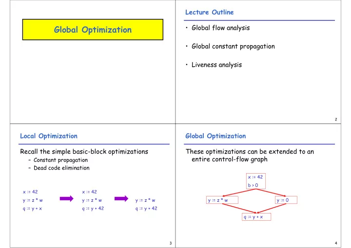
Lecture Outline • Global flow analysis Global Optimization • Global constant propagation • Liveness analysis 2 Local Optimization Global Optimization Recall the simple basic-block optimizations These optimizations can be extended to an entire control-flow graph – Constant propagation – Dead code elimination x := 42 b > 0 x := 42 x := 42 y := z * w y := z * w y := z * w y := z * w y := 0 q := y + x q := y + 42 q := y + 42 q := y + x 3 4

Global Optimization Global Optimization These optimizations can be extended to an These optimizations can be extended to an entire control-flow graph entire control-flow graph x := 42 x := 42 b > 0 b > 0 y := z * w y := 0 y := z * w y := 0 q := y + x q := y + 42 5 6 Correctness Correctness (Cont.) • How do we know whether it is OK to globally To replace a use of x by a constant k we must propagate constants? know that the following property ** holds: • There are situations where it is incorrect: On every path to the use of x, x := 42 the last assignment to x is x := k ** b > 0 y := z * w y := 0 x := 54 q := y + x 7 8

Example 1 Revisited Example 2 Revisited x := 42 x := 42 b > 0 b > 0 y := z * w y := 0 y := z * w y := 0 x := 54 q := y + x q := y + x 9 10 Discussion Global Analysis • The correctness condition is not trivial to Global optimization tasks share several traits: check – The optimization depends on knowing a property P at a particular point in program execution – Proving P at any point requires knowledge of the • “All paths” includes paths around loops and entire function body through branches of conditionals – It is OK to be conservative: If the optimization requires P to be true, then want to know either • Checking the condition requires global analysis • that P is definitely true, or • that we don’t know whether P is true – An analysis that determines how data flows over the entire control-flow graph – It is always safe to say “don’t know” 11 12

Global Analysis (Cont.) Global Constant Propagation • Global dataflow analysis is a standard • Global constant propagation can be performed technique for solving problems with these at any point where property ** holds characteristics • Consider the case of computing ** for a single • Global constant propagation is one example of variable x at all program points an optimization that requires global dataflow analysis 13 14 Global Constant Propagation (Cont.) Example • To make the problem precise, we associate one of the following values with x at every program point x = * x := 42 x = 42 b > 0 value interpretation x = 42 x = 42 This statement never executes # y := z * w y := 0 x = 42 c x = constant c x := 54 x = 42 x = 54 x = * * Don’t know whether x is a constant q := y + x x = * 15 16

Using the Information The Analysis Idea • Given global constant information, it is easy to perform the optimization – Simply inspect the x = ? associated with a The analysis of a (complicated) program can be statement using x expressed as a combination of simple rules – If x is constant at that point replace that use of x relating the change in information between by the constant adjacent statements • But how do we compute the properties x = ? 17 18 Explanation Transfer Functions • The idea is to “push” or “transfer” information • Define a transfer function that transfers from one statement to the next information from one statement to another • For each statement s, we compute information • In the following rules, let statement s have as about the value of x immediately before and immediate predecessors statements p 1 ,…,p n after s C in (x,s) = value of x before s C out (x,s) = value of x after s 19 20

Rule 1 Rule 2 x = * x = d x = ? x = ? x = ? x = c x = ? x = ? x = * x = * s s if C out (x, p i ) = * for any i, then C in (x, s) = * If C out (x, p i ) = c and C out (x, p j ) = d and d ≠ c then C in (x, s) = * 21 22 Rule 3 Rule 4 x = c x = # x = # x = # x = c x = # x = # x = # x = c x = # s s if C out (x, p i ) = c or # for all i, if C out (x, p i ) = # for all i, then C in (x, s) = c then C in (x, s) = # 23 24

The Other Half Rule 5 • Rules 1-4 relate the out of one statement to the in of the successor statement x = # s • We also need rules relating the in of a x = # statement to the out of the same statement C out (x, s) = # if C in (x, s) = # 25 26 Rule 6 Rule 7 x = ? x = ? x := c x := f(…) x = c x = * C out (x, x := c) = c if c is a constant C out (x, x := f(…)) = * This rule says that we do not perform inter-procedural analysis (i.e. we do not look at what other functions do) 27 28

Rule 8 An Algorithm 1. For every entry s to the function, set C in (x, s) = * x = a y := . . . 2. Set C in (x, s) = C out (x, s) = # everywhere else x = a 3. Repeat until all points satisfy 1-8: Pick s not satisfying 1-8 and update using the appropriate rule C out (x, y := …) = C in (x, y := …) if x ≠ y 29 30 The Value # Discussion To understand why we need #, look at a loop • Consider the statement y := 0 • To compute whether x is constant at this point, we need to know whether x is constant x = * x := 42 at the two predecessors x = 42 b > 0 – x := 42 x = 42 x = 42 – q := y + x y := z * w y := 0 x = 42 • But information for q := y + x depends on its predecessors, including y := 0! q := y + x q < b 31 32

The Value # (Cont.) Example • Because of cycles, all points must have values at all times x = * x := 42 x = 42 b > 0 x = 42 • Intuitively, assigning some initial value allows x = 42 the analysis to break cycles y := z * w y := 0 x = 42 x = # x = # • The initial value # means “So far as we know, q := x + y x = # control never reaches this point” q < b 33 34 Example Example x = * x = * x := 42 x := 42 x = 42 x = 42 b > 0 b > 0 x = 42 x = 42 x = 42 x = 42 y := z * w y := 0 y := z * w y := 0 x = 42 x = 42 x = # x = # x = 42 x = 42 q := x + y q := x + y x = # x = 42 q < b q < b 35 36

Example Orderings • We can simplify the presentation of the x = * analysis by ordering the values x := 42 x = 42 # < c < * b > 0 x = 42 x = 42 y := z * w y := 0 • Drawing a picture with “lower” values drawn lower, we get x = 42 x = 42 x = 42 * q := x + y x = 42 q < b -1 0 1 ... ... # 37 38 Orderings (Cont.) Termination • * is the greatest value, # is the least • Simply saying “repeat until nothing changes” doesn’t guarantee that eventually we reach a – All constants are in between and incomparable point where nothing changes • Let lub be the least-upper bound in this • The use of lub explains why the algorithm ordering terminates – Values start as # and only increase • Rules 1-4 can be written using lub: – # can change to a constant, and a constant to * C in (x, s) = lub { C out (x, p) | p is a predecessor of s } – Thus, C_(x, s) can change at most twice 39 40

Termination (Cont.) Liveness Analysis Thus the algorithm is linear in program size Once constants have been globally propagated, we would like to eliminate dead code Number of steps = x := 42 b > 0 Number of C_(….) values computed * 2 = Number of program statements * 4 y := z * w y := 0 q := y + x After constant propagation, x := 42 is dead (assuming x is not used elsewhere) 41 42 Live and Dead Variables Liveness • The first value of x is x := 42 A variable x is live at statement s if dead (never used) – There exists a statement s’ that uses x • The second value of x is – There is a path from s to s’ x := 54 live (may be used) – That path has no intervening assignment to x • Liveness is an important concept for the compiler y := x 43 44

Global Dead Code Elimination Computing Liveness • A statement x := … is dead code if x is dead • We can express liveness in terms of after the assignment information transferred between adjacent statements, just as in copy propagation • Dead statements can be deleted from the program • Liveness is simpler than constant propagation, since it is a boolean property (true or false) • But we need liveness information first . . . 45 46 Liveness Rule 1 Liveness Rule 2 p x = true x = true …:= f(x) x = ? x = ? x = ? x = true x = ? L in (x, s) = true if s refers to x on the RHS (x, p) = ∨ L out { L in (x, s) | s a successor of p } 47 48

Liveness Rule 3 Liveness Rule 4 x = false x = a x := e s x = ? x = a L in (x, x := e) = false if e does not refer to x L in (x, s) = L out (x, s) if s does not refer to x 49 50 Algorithm Termination 1. Let all L_(…) = false initially • A value can change from false to true, but not the other way around 2. Repeat until all statements s satisfy rules 1-4 • Each value can change only once, so Pick s where one of 1-4 does not hold and termination is guaranteed update using the appropriate rule • Once the analysis information is computed, it is simple to eliminate dead code 51 52