SLIDE 1 Geometric Methods in Representation Theory Columbia, Missouri, November 23-25, 2014 Varieties of Invariant Subspaces
Markus Schmidmeier (Florida Atlantic University)
. . . . . . . . . . . . . . . . . . . . . . . . . . . . . . . . . . . . . . . . . . . . . . . . . . . . . . . . . . . . . . . . . . . . . . . . . . . . . . . . . . . . . . . . . . . . . . . . . . . . . . . . . . . . . . . . . . . . . . . . . . . . . . . . . . . . . . . . . . . . . . . . . . . . . . . . . . . . . . . . . . . . . . . . . . . . . . . . . . . . . . . . . . . . . . . . . . . . . . . . . . . . . . . . . . . . . . . . . . . . . . . . . . . . . . . . . . . . . . . . . . . . . . . . . . . . . . . . . . ϕ . . . . . . . . . . . . . . . . . . . . . . . . . . . . . .................... . . . . . . . . . . . . . . . . . . . . . . . . . . . . . . . . . . . . . . . . . . . . . . . . . . . . . . . . . . . . . . . . . . . . . . . . . . . . . . . . . . . . . . . . . . . . . . . . . . . . . . . . . . . . . . . . . . . . . . . . . . . . . . . . . . . . . . . . . . . . . . . . . . . . . . . . . . . . . . . . . . . . . .
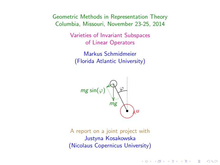
mg sin(ϕ) mg
. . . . . . . . . . . . . . . . . . . . . . . . . . . . . . . . . . . . . . . . . . . . . . . . . . . . . . . . . . . . . . . . . . . . . . . . . . . . . . . . . . . . . . . . . . . . . . . . . . . . . . . . . . . . . . . . . . . . . . . . . . . . . . . . . . . . . . . . . . . . . . . . . . . . . . . . . . . . . . . . . . . . . . . . . . . . . . . . . . . . . . . . . . . . . . . . . . . . . . . . . . . . . . . . . . . . . u
A report on a joint project with Justyna Kosakowska (Nicolaus Copernicus University)
SLIDE 2 Short exact sequences of nilpotent linear operators
Definition: For α a partition and k a field, we denote the nilpotent linear operator of type α by Nα =
k[T]/(T αi). For fixed partitions α, β, γ, we are interested in short exact sequences of nilpotent linear operators 0 − → Nα
f
− → Nβ − → Nγ − → 0 Definition: Vβ
α,γ = {f : Nα → Nβ | Cok(f ) ∼
= Nγ} Vβ
α,γ is a constructible subset of the affine variety Homk(Nα, Nβ).
SLIDE 3 Aim
◮ Motivation I: Varieties of type Vβ α,γ occur in a applications. ◮ Motivation II: They are interesting geometrically. ◮ The components: Study the partition
Vβ
α,γ =
- Γ LR-tableau of shape (α, β, γ)
VΓ
α,γ into irreducible components VΓ. ◮ The relation: Introduce the closure relation V˜ Γ ∩ VΓ = ∅ to
see how the components are linked.
◮ Example: Review the case α1 ≤ 2 (all parts of α are at most
2).
◮ Main result: Compare this relation on the set of LR-tableaux
- f shape (α, β, γ) with combinatorial relations ≤box, ≤part and
algebraic relations ≤ext, ≤hom.
◮ Part of the proof: Show that ≤closure implies ≤part.
SLIDE 4
Motivation I: Control Systems
A linear time invariant dynamical system Σ is given by the differential equations Σ : dx
dt
= Bx + Au y = Cx where u(t) ∈ Cm is the input or control x(t) ∈ Cn the state and y(t) ∈ Cp the output at time t.
SLIDE 5
Motivation I: Control Systems
A linear time invariant dynamical system Σ is given by the differential equations Σ : dx
dt
= Bx + Au y = Cx where u(t) ∈ Cm is the input or control x(t) ∈ Cn the state and y(t) ∈ Cp the output at time t. Time invariance means that A ∈ Cn×m, B ∈ Cn×n, and C ∈ Cp×n, so we are dealing with a linear representation: Σ : Cm
·A
− → ·B Cn
·C
− → Cp
SLIDE 6 Motivation I: Inverted Pendulum
In every text book on control theory, you will find this example.
. . . . . . . . . . . . . . . . . . . . . . . . . . . . . . . . . . . . . . . . . . . . . . . . . . . . . . . . . . . . . . . . . . . . . . . . . . . . . . . . . . . . . . . . . . . . . . . . . . . . . . . . . . . . . . . . . . . . . . . . . . . . . . . . . . . . . . . . . . . . . . . . . . . . . . . . . . . . . . . . . . . . . . . . . . . . . . . . . . . . . . . . . . . . . . . . . . . . . . . . . . . . . . . . . . . . . . . . . . . . . . . . . . . . . . . . . . . . . . . . . . . . . . . . . . . . . . . . . . ϕ . . . . . . . . . . . . . . . . . . . . . . . . . . . . . .................... . . . . . . . . . . . . . . . . . . . . . . . . . . . . . . . . . . . . . . . . . . . . . . . . . . . . . . . . . . . . . . . . . . . . . . . . . . . . . . . . . . . . . . . . . . . . . . . . . . . . . . . . . . . . . . . . . . . . . . . . . . . . . . . . . . . . . . . . . . . . . . . . . . . . . . . . . . . . . . . . . . . . . .
mg sin(ϕ) mg
. . . . . . . . . . . . . . . . . . . . . . . . . . . . . . . . . . . . . . . . . . . . . . . . . . . . . . . . . . . . . . . . . . . . . . . . . . . . . . . . . . . . . . . . . . . . . . . . . . . . . . . . . . . . . . . . . . . . . . . . . . . . . . . . . . . . . . . . . . . . . . . . . . . . . . . . . . . . . . . . . . . . . . . . . . . . . . . . . . . . . . . . . . . . . . . . . . . . . . . . . . . . . . . . . . . . . u
SLIDE 7 Motivation I: Inverted Pendulum
In every text book on control theory, you will find this example.
. . . . . . . . . . . . . . . . . . . . . . . . . . . . . . . . . . . . . . . . . . . . . . . . . . . . . . . . . . . . . . . . . . . . . . . . . . . . . . . . . . . . . . . . . . . . . . . . . . . . . . . . . . . . . . . . . . . . . . . . . . . . . . . . . . . . . . . . . . . . . . . . . . . . . . . . . . . . . . . . . . . . . . . . . . . . . . . . . . . . . . . . . . . . . . . . . . . . . . . . . . . . . . . . . . . . . . . . . . . . . . . . . . . . . . . . . . . . . . . . . . . . . . . . . . . . . . . . . . ϕ . . . . . . . . . . . . . . . . . . . . . . . . . . . . . .................... . . . . . . . . . . . . . . . . . . . . . . . . . . . . . . . . . . . . . . . . . . . . . . . . . . . . . . . . . . . . . . . . . . . . . . . . . . . . . . . . . . . . . . . . . . . . . . . . . . . . . . . . . . . . . . . . . . . . . . . . . . . . . . . . . . . . . . . . . . . . . . . . . . . . . . . . . . . . . . . . . . . . . .
mg sin(ϕ) mg
. . . . . . . . . . . . . . . . . . . . . . . . . . . . . . . . . . . . . . . . . . . . . . . . . . . . . . . . . . . . . . . . . . . . . . . . . . . . . . . . . . . . . . . . . . . . . . . . . . . . . . . . . . . . . . . . . . . . . . . . . . . . . . . . . . . . . . . . . . . . . . . . . . . . . . . . . . . . . . . . . . . . . . . . . . . . . . . . . . . . . . . . . . . . . . . . . . . . . . . . . . . . . . . . . . . . . u
After linearization, the differential equation m ¨ ϕ = mg sin(ϕ) + u becomes m ¨ ϕ = mgϕ + u. So the assignments x = ϕ ˙ ϕ
y = ϕ, u = u lead to the dynamical system Σ :
dt
= 0 1
g 0
1/m
y = (1 0) · x Challenge: Apply torque u to bring and keep the pendulum in the vertical position.
SLIDE 8 Motivation I: The Kalman Decomposition
A linear time-invariant dynamical system Σ : Vin
a
− → T V
c
− → Vout gives rise to two T-invariant subspaces of V : VC =
the controlable subspace V ¯
O
=
the non-observable subspace
SLIDE 9 Motivation I: The Kalman Decomposition
A linear time-invariant dynamical system Σ : Vin
a
− → T V
c
− → Vout gives rise to two T-invariant subspaces of V : VC =
the controlable subspace V ¯
O
=
the non-observable subspace The Kalman embedding VC ∩ V ¯
O ⊂ VC ⊂
invariant subspaces. Putting VK = VC/VC ∩ V ¯
O, we obtain a completely controlable
and completely observable system, the minimal realisation: Σmin : Vin
¯ a
− → ¯
T
VK
¯ c
− → Vout
SLIDE 10 Motivation II: Arbitrary Operators
Suppose v, u are natural numbers with 0 ≤ u ≤ v and V is a (complex) vector space of dimension v. Observations:
- 1. Generically, a linear operator T : V → V decomposes as the
direct sum of v linear operators, each acting with a different eigen value on a one-dimensional eigen space.
- 2. Each T -invariant subspace U of V of dimension u is
determined by a subset of u elements of the set of eigen values. · · · · · ·
E(λu) E(λu+1) E(λv)
- 3. In this sense, “Semisimple is dense”.
SLIDE 11 Motivation II: Nilpotent Operators
Suppose that v, u are natural numbers with 0 ≤ u ≤ v, that V is a vector space of dimension v, and that T : V → V acts nilpotently. Observations:
- 1. Generically, a nilpotent linear operator T : V → V has only
- ne Jordan block of size v corresponding to the eigen value 0.
- 2. In this case, there is a unique T -invariant subspace U of V of
dimension u. Pv
u :
. . . . . .
v
x
B = (V , T) = x k[T]/(T v) A = (U, T) = (x T v−u)
- 3. In this case, the embedding (A ⊂ B) is a “picket” since the
ambient space B is a uniserial module. “Pickets are dense”.
SLIDE 12 Motivation II: Operators with fixed Jordan type
Let α, β, γ be partitions. Observations:
- 1. The operators Nα, Nβ, Nγ are determined uniquely, up to
isomorphism, by the partitions.
- 2. The number of irreducible components in Vβ
α,γ is given by the
Littlewood-Richardson coefficient cβ
α,γ.
SLIDE 13 Motivation II: Operators with fixed Jordan type
Let α, β, γ be partitions. Observations:
- 1. The operators Nα, Nβ, Nγ are determined uniquely, up to
isomorphism, by the partitions.
- 2. The number of irreducible components in Vβ
α,γ is given by the
Littlewood-Richardson coefficient cβ
α,γ.
Recall: The LR-coefficient features prominently in many exciting algebraic problems:
◮ Multiplication of Schur polynomials ◮ Eigenvalues of sums of Hermitian matrices ◮ Number of points in intersection of Schubert varieties ◮ Leading coefficient of the Hall polynomial
Combinatorially, cβ
α,γ counts the LR-tableaux of shape (α, β, γ).
SLIDE 14
The components: LR-tableaux
Definition: An LR-tableau of shape (α, β, γ) is a Young diagram of shape β in which the region β \ γ contains α′
1 entries 1 , ..., α′ s entries s ,
where s = α1 is the largest entry, such that
◮ in each row, the entries are weakly increasing, ◮ in each column, the entries are strictly increasing, ◮ for each ℓ > 1 and each column c: on the right hand side of c,
the number of entries ℓ − 1 is at least the number of entries ℓ. Example: Let α = (211), β = (4321), γ = (321); then α′ = (31). Γ :
1 2 1 1
Γ = [321, 4221, 4321] Notation: Write Γ = [γ(0), . . . , γ(s)] where γ(i) denotes the region in the Young diagram β which contains the entries , 1 , ... , i .
SLIDE 15 The components: The LR-tableau of an embedding
Theorem (Green and Klein, 1968): There exists a short exact sequence 0 − → Nα − → Nβ − → Nγ − → 0 if and only if there exists an LR-tableau of shape (α, β, γ). Definition: The LR-tableau Γ of an embedding A ⊂ B is given by Γ = [γ(i)]i=0,...,s, where s = α1 and γ(i) = type B/T iA. Property: Vβ
α,γ =
- Γ LR-tableau of shape (α, β, γ)
VΓ where the VΓ = {f : Nα → Nβ | f has LR-tableau Γ} are Glα × Glβ-invariant irreducible varieties of the same dimension.
SLIDE 16
The relation: The closure relation for LR-tableaux
Definition: For partitions α, β, γ, we denote by T β
α,γ the set of all
LR-tableaux of shape (α, β, γ). We are interested how the varieties VΓ, Γ ∈ T β
α,γ, are linked.
Definition: For LR-tableaux Γ, ˜ Γ ∈ T β
α,γ we write Γ≤closure˜
Γ if V˜
Γ ∩ VΓ = ∅.
Remark: The closure relation is a pre-order (i.e. reflexive and antisymmetric) as we will see. In general, ≤closure is not transitive. Definition: We denote by ≤∗
closure the transitive closure.
SLIDE 17 Example: The variety V4321
211,321
∆6 :
1 1 1 21
❅ ❅ ❅ ❅ ■
∆4 :
1 1 1 22
∆5 :
1 1 21 1
✻ ✻
∆1 :
1 1 1 23
∆3 :
1 21 1 1
❅ ❅ ❅ ❅ ■
∆2 :
1 1 22 1
dim = 12 dim = 11 dim = 13
SLIDE 18 Example: The variety V4321
211,321
∆6 :
3 2 1
✤ ✜
❅ ❅ ❅ ❅ ■
∆4 :
3 2 1
✓ ✏
∆5 :
3 2 1
✓ ✏ ✻ ✻
∆1 :
3 2 1
✞ ☎
∆3 :
3 2 1
✞ ☎
❅ ❅ ❅ ❅ ■
∆2 :
3 2 1
✞ ☎
dim = 12 dim = 11 dim = 13
SLIDE 19 Example: The variety V4321
211,321
∆6 :
❅ ❅ ❅ ❅ ■
∆4 :
✻
∆1 :
❅ ❅ ❅ ❅ ■
∆2 :
dim = 12 dim = 11 dim = 13
SLIDE 20
Main result: The combinatorial orders
Definition: Let T β
α,γ be the set of all LR-tableaux of shape (α, β, γ).
Recall that there is a natural partial ordering for partitions given by α≤partβ if for all j, j
i=0 αi ≥ j i=0 βi.
Definition: For LR-tableaux Γ = [γ(0), . . . , γ(s)], ˜ Γ = [˜ γ(0), . . . , ˜ γ(s)], we say Γ ≤part ˜ Γ if for each i, γ(i)≤part˜ γ(i). Example:
1 1 1 2
>part
1 1 2 1
>part
1 2 1 1 [321,3321,4321] [321,4221,4321] [321,4311,4321]
SLIDE 21 Main result: The combinatorial orders
Definition: Let T β
α,γ be the set of all LR-tableaux of shape (α, β, γ).
Recall that there is a natural partial ordering for partitions given by α≤partβ if for all j, j
i=0 αi ≥ j i=0 βi.
Definition: For LR-tableaux Γ = [γ(0), . . . , γ(s)], ˜ Γ = [˜ γ(0), . . . , ˜ γ(s)], we say Γ ≤part ˜ Γ if for each i, γ(i)≤part˜ γ(i). Example:
1 1 1 2
>part
1 1 2 1
>part
1 2 1 1 [321,3321,4321] [321,4221,4321] [321,4311,4321]
Definition: By ≤box we denote the transitive closure of the relation
α,γ given by exchanging two boxes such that the smaller entry
moves up. Theorem: ≤box implies ≤∗
closure implies ≤part.
SLIDE 22
Main result: The algebraic orders
For Γ, ˜ Γ ∈ T β
α,γ define: ◮ Γ ≤ext ˜
Γ, if there are X ∈ VΓ, ˜ X ∈ V˜
Γ with X ≤ext ˜
X, (In particular, X ≤ext ˜ X if ˜ X = ˜ X1 ⊕ ˜ X2 and there is a short exact sequence 0 → ˜ X1 → X → ˜ X2 → 0.)
◮ Γ ≤deg ˜
Γ, if there are X, ˜ X such that X ≤deg ˜ X. (Recall X ≤deg ˜ X if O ˜
X ⊂ OX.) ◮ Γ ≤hom ˜
Γ, if there are X, ˜ X with X ≤hom ˜ X, (equivalently, for all T, dim Hom(X, T) ≤ dim Hom( ˜ X, T).
SLIDE 23
Main result: The algebraic orders
For Γ, ˜ Γ ∈ T β
α,γ define: ◮ Γ ≤ext ˜
Γ, if there are X ∈ VΓ, ˜ X ∈ V˜
Γ with X ≤ext ˜
X, (In particular, X ≤ext ˜ X if ˜ X = ˜ X1 ⊕ ˜ X2 and there is a short exact sequence 0 → ˜ X1 → X → ˜ X2 → 0.)
◮ Γ ≤deg ˜
Γ, if there are X, ˜ X such that X ≤deg ˜ X. (Recall X ≤deg ˜ X if O ˜
X ⊂ OX.) ◮ Γ ≤hom ˜
Γ, if there are X, ˜ X with X ≤hom ˜ X, (equivalently, for all T, dim Hom(X, T) ≤ dim Hom( ˜ X, T). Note 1: As for modules, ≤ext implies ≤deg implies ≤hom. Note 2: Since O ˜
X ⊂ V˜ Γ and OX ⊂ VΓ, ≤deg implies ≤closure.
Theorem: ≤ext implies ≤closure implies ≤hom−pic (the restriction of ≤hom to pickets T).
SLIDE 24
Main result: How the partial orders are related
Theorem: For LR-tableaux Γ, ˜ Γ of the same shape, the following implications hold. ≤part ≤∗
hom
≤∗
closure
≤∗
deg
≤∗
ext
≤box ↓ ↓ ւ ց ց ւ
SLIDE 25
Main result: How the partial orders are related
Theorem: For LR-tableaux Γ, ˜ Γ of the same shape, the following implications hold. ≤part ≤∗
hom
≤∗
closure
≤∗
deg
≤∗
ext
≤box ↓ ↓ ւ ց ց ւ Corollary: The closure relation is a partial order controlled combinatorially and algebraically (note ≤part is equivalent to ≤hom−pic).
SLIDE 26
Main result: How the partial orders are related
Theorem: For LR-tableaux Γ, ˜ Γ of the same shape, the following implications hold. ≤part ≤∗
hom
≤∗
closure
≤∗
deg
≤∗
ext
≤box ↓ ↓ ւ ց ց ւ Corollary: The closure relation is a partial order controlled combinatorially and algebraically (note ≤part is equivalent to ≤hom−pic). Theorem (KS 2012): Suppose α is a partition with all parts at most 2. All partially ordered sets are equivalent.
SLIDE 27
Proof: The closure relation implies the part relation, always
Theorem: If V˜
Γ ∩ VΓ = ∅ then Γ ≤part ˜
Γ. Proof: We assume Γ≤part˜ Γ to define a closed subset U ⊂ Vβ
α,γ
such that the following conditions hold: VΓ ⊂ U and U ∩ V˜
Γ = ∅
SLIDE 28
Proof: The closure relation implies the part relation, always
Theorem: If V˜
Γ ∩ VΓ = ∅ then Γ ≤part ˜
Γ. Proof: We assume Γ≤part˜ Γ to define a closed subset U ⊂ Vβ
α,γ
such that the following conditions hold: VΓ ⊂ U and U ∩ V˜
Γ = ∅
For the closure of U we use the following Lemma: Suppose M is a set of monomorphisms between vector spaces A, B. For subspaces U ⊂ A, V ⊂ B, and for n ∈ N, the condition dim(f (U) ∩ V ) ≥ n defines a closed subset in M. Proof:
◮ The condition rank(f ) > m defines an open subset in
Hom(A, B)
◮ The condition dim f (U)+V V
> m defines an open subset in Hom(A, B)
◮ The subset defined by dim f (U) f (U)∩V > m is open ◮ On M, the subset given by dim(f (U) ∩ V ) < n is open
SLIDE 29
Summary
◮ Set-Up: Given partitions α, β, γ, the short exact sequences
0 → Nα → Nβ → Nγ → 0 form a constructible subset Vβ
α,γ of
an affine variety.
◮ Motivation: Varieties of type Vβ α,γ occur in applications and
are of interest geometrically.
◮ Fact: Each variety Vβ α,γ has cβ α,γ irreducible components VΓ
where cβ
α,γ is the Littlewood-Richardson coefficient. ◮ Aim: Study the closure relation given by V˜ Γ ∩ VΓ = ∅. ◮ Example: In case α1 ≤ 2, the closure relation is known. ◮ Main result: The closure relation is under control
combinatorially (≤box implies ≤∗
closure implies ≤part) and
algebraically (≤∗
ext implies ≤∗ closure implies ≤hom−pic). ◮ Proof: We showed the Key-Lemma for ≤∗ closure implies ≤part.
SLIDE 30
Summary
◮ Set-Up: Given partitions α, β, γ, the short exact sequences
0 → Nα → Nβ → Nγ → 0 form a constructible subset Vβ
α,γ of
an affine variety.
◮ Motivation: Varieties of type Vβ α,γ occur in applications and
are of interest geometrically.
◮ Fact: Each variety Vβ α,γ has cβ α,γ irreducible components VΓ
where cβ
α,γ is the Littlewood-Richardson coefficient. ◮ Aim: Study the closure relation given by V˜ Γ ∩ VΓ = ∅. ◮ Example: In case α1 ≤ 2, the closure relation is known. ◮ Main result: The closure relation is under control
combinatorially (≤box implies ≤∗
closure implies ≤part) and
algebraically (≤∗
ext implies ≤∗ closure implies ≤hom−pic). ◮ Proof: We showed the Key-Lemma for ≤∗ closure implies ≤part.
Thank You!