Genomic sequence analysis: - - PDF document

Genomic ¡sequence ¡analysis: ¡ gene ¡predic4on

We ¡want ¡to ¡know ¡how ¡this…

TGCATCGATCGTAGCTAGCTAGCGCATGCTAGCTAGCTAGCTAGCTACGATGCATCG TGCATCGATCGATGCATGCTAGCTAGCTAGCTAGCATGCTAGCTAGCTAGCTATTGG CGCTAGCTAGCATGCATGCATGCATCGATGCATCGATTATAAGCGCGATGACGTCAG CGCGCGCATTATGCCGCGGCATGCTGCGCACACACAGTACTATAGCATTAGTAAAAA GGCCGCGTATATTTTACACGATAGTGCGGCGCGGCGCGTAGCTAGTGCTAGCTAGTC TCCGGTTACACAGGTAGCTAGCTAGCTGCTAGCTAGCTGCTGCATGCATGCATTAGT AGCTAGTGTAGCTAGCTAGCATGCTGCTAGCATGCAGCATGCATCGGGCGCGATGCT GCTAGCGCTGCTAGCTAGCTAGCTAGCTAGGCGCTAATTATTTATTTTGGGGGGTTA AAAAAAAAAATTTCGCTGCTTATACCCCCCCCCACATGATGATCGTTAGTAGCTACT AGCTCTCATCGCGCGGGGGGATGCTTAGCGTGGTGTGTGTGTGTGGTGTGTGTGGTC CTATAATTAGTGCATCGGCGCATCGATGGCTAGTCGATCGATCGATTTTATATATCT AAAGACCCCATCTCTCTCTCTTTTCCCTTCTCTCGCTAGCGGGCGGTACGATTTACC GGCCGCGTATATTTTACACGATAGTGCGGCGCGGCGCGTAGCTAGTGCTAGCTAGTC AGCTCTCATCGCGCGGGGGGATGCTTAGCGTGGTGTGTGTGTGTGGTGTGTGTGGTC TGCATCGATCGATGCATGCTAGCTAGCTAGCTAGCATGCTAGCTAGCTAGCTATTGG CTATAATTAGTGCATCGGCGCATCGATGGCTAGTCGATCGATCGATTTTATATATCT CGCTAGCTAGCATGCATGCATGCATCGATGCATCGATTATAAGCGCGATGACGTCAG TCCGGTTACACAGGTAGCTAGCTAGCTGCTAGCTAGCTGCTGCATGCATGCATTAGT

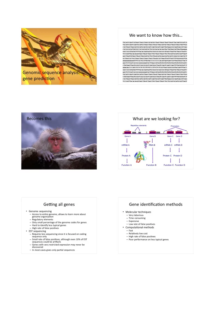
Becomes ¡this What ¡are ¡we ¡looking ¡for?

Protein A Protein C Protein D Function A Function B Function C Function D

Gene A Gene B Gene C Gene D Repetitive elements Promoters

mRNA A RNA B mRNA C mRNA D

Ge>ng ¡all ¡genes

• Genome ¡sequencing

– Access ¡to ¡en4re ¡genome, ¡allows ¡to ¡learn ¡more ¡about ¡ genome ¡organiza4on – Regulatory ¡elements – Only ¡small ¡percentage ¡of ¡the ¡genome ¡codes ¡for ¡genes – Hard ¡to ¡iden4fy ¡less ¡typical ¡genes – High ¡rate ¡of ¡false ¡posi4ves

• EST ¡sequencing

– Requires ¡less ¡sequencing ¡since ¡it ¡is ¡focused ¡on ¡coding ¡ sequence ¡only – Small ¡rate ¡of ¡false ¡posi4ves, ¡although ¡even ¡10% ¡of ¡EST ¡ sequences ¡could ¡be ¡ar4facts – Genes ¡with ¡very ¡restricted ¡expression ¡may ¡never ¡be ¡ discovered – In ¡most ¡cases ¡gives ¡only ¡par4al ¡sequences

Gene ¡iden4fica4on ¡methods

• Molecular ¡techniques

– Very ¡laborious – Time ¡consuming – Expensive – Low ¡rate ¡of ¡false ¡posi4ves

• Computa4onal ¡methods

– Fast – Rela4vely ¡low ¡cost – High ¡rate ¡of ¡false ¡posi4ves – Poor ¡performance ¡on ¡less ¡typical ¡genes

Genome ¡sequencing

Shotgun Sequencing Clone into vector Assembly

Shotgun ¡sequencing ¡is ¡ the ¡method ¡of ¡choice ¡ for ¡small ¡genomes Repe66ve ¡sequences ¡make ¡ correct ¡assembly ¡difficult

Clone-­‑by-­‑clone ¡approach Before ¡we ¡start ¡analysis…

• We ¡have ¡to:

– Check ¡sequences ¡quality – Remove ¡contamina4on – Assembly ¡sequence ¡reads ¡into ¡longer ¡con4gs – Close ¡gaps ¡(in ¡perfect ¡situa4on)

Gene ¡finding ¡methods ¡classifica4on

Similarity based predictors: make use of similarity to already known genes and proteins coded by these genes as well as expression data including sequences from cDNAs and data from hybridization experiments (tiling arrays for example) Dual- and multi-genome predictors: rely on the fact that functional regions

• f a genome sequence are more

conserved during evolution Model based predictors: use a single genome sequence and exon/ intron structure is predicted based

• n absolute and bulk properties of

the sequence

Similarity ¡search

• We ¡can ¡check ¡if ¡any ¡fragment ¡of ¡our ¡sequence

¡ shows ¡similarity ¡to ¡already ¡known ¡protein. ¡We ¡ can ¡also ¡check ¡if ¡there ¡are ¡any ¡mRNA ¡ sequences ¡and ¡ESTs ¡which ¡align ¡well ¡with ¡the ¡ genomic ¡sequence. ¡Based ¡on ¡similarity ¡we ¡can ¡ deduct ¡the ¡gene ¡structure ¡and ¡protein ¡ func4on

Comparative genomics - Comparative genomics - MultiPipMaker MultiPipMaker

http://pipmaker.bx.psu.edu/pipmaker/

Model ¡based ¡methods

• We ¡take ¡advantage ¡of ¡what ¡we ¡already

¡ learned ¡about ¡gene ¡structures ¡and ¡features ¡of ¡ coding ¡sequences. ¡Based ¡on ¡this ¡knowledge ¡ we ¡can ¡build ¡theore4cal ¡model, ¡develop ¡an ¡ algorithm ¡to ¡search ¡for ¡important ¡features, ¡ train ¡it ¡on ¡known ¡data ¡and ¡use ¡to ¡search ¡for ¡ coding ¡sequences ¡in ¡anonymous ¡genomic ¡ fragments All ¡informa4on ¡is ¡in ¡the ¡DNA. ¡We ¡just ¡have ¡to ¡ learn ¡how ¡to ¡read ¡the ¡code, ¡the ¡program ¡for ¡life.

TGCATCGATCGTAGCTAGCTAGCGCATGCTAGCTAGCTAGCTAGCTACGATGCATCG TGCATCGATCGATGCATGCTAGCTAGCTAGCTAGCATGCTAGCTAGCTAGCTATTGG CGCTAGCTAGCATGCATGCATGCATCGATGCATCGATTATAAGCGCGATGACGTCAG CGCGCGCATTATGCCGCGGCATGCTGCGCACACACAGTACTATAGCATTAGTAAAAA GGCCGCGTATATTTTACACGATAGTGCGGCGCGGCGCGTAGCTAGTGCTAGCTAGTC TCCGGTTACACAGGTAGCTAGCTAGCTGCTAGCTAGCTGCTGCATGCATGCATTAGT AGCTAGTGTAGCTAGCTAGCATGCTGCTAGCATGCAGCATGCATCGGGCGCGATGCT GCTAGCGCTGCTAGCTAGCTAGCTAGCTAGGCGCTAATTATTTATTTTGGGGGGTTA AAAAAAAAAATTTCGCTGCTTATACCCCCCCCCACATGATGATCGTTAGTAGCTACT AGCTCTCATCGCGCGGGGGGATGCTTAGCGTGGTGTGTGTGTGTGGTGTGTGTGGTC CTATAATTAGTGCATCGGCGCATCGATGGCTAGTCGATCGATCGATTTTATATATCT AAAGACCCCATCTCTCTCTCTTTTCCCTTCTCTCGCTAGCGGGCGGTACGATTTACC

Program ¡for ¡life

• DNA ¡in ¡our ¡cells ¡store ¡informa4on ¡in ¡a ¡way ¡that ¡is ¡very ¡similar ¡to ¡the ¡way ¡computers ¡do.
• Instead ¡of ¡being ¡a ¡binary ¡memory, ¡where ¡everything ¡is ¡either ¡0 ¡or ¡1, ¡DNA ¡is ¡a ¡4 ¡le]er

¡ alphabet: ¡A, ¡C, ¡G, ¡T

• Using ¡computer ¡metaphor ¡we ¡can ¡say ¡that:

– Plant ¡cell ¡do ¡not ¡look ¡like ¡a ¡mouse ¡cell ¡because ¡their ¡“programs” ¡are ¡different – Liver ¡cells ¡work ¡differently ¡than ¡lung ¡cells ¡because ¡of ¡different ¡input ¡to ¡the ¡program

¡

– Children ¡look ¡like ¡parents ¡because ¡their ¡program ¡is ¡a ¡“revision” ¡of ¡parents ¡program – Many ¡diseases ¡are ¡caused ¡by ¡“bugs” ¡in ¡program:

• Familial ¡dysautonomia: ¡A ¡simple ¡mistake ¡in ¡one ¡line ¡of ¡code
• Hun4ngton’s ¡disease: ¡A ¡“line” ¡of ¡code ¡gets ¡repeated ¡a ¡bunch ¡of ¡4mes ¡by ¡

accident

• Different ¡ways ¡to ¡solve ¡the ¡same ¡problem:

– Plants: ¡photosynthesis ¡= ¡turn ¡light ¡into ¡sugar – Animals: ¡eat ¡plant ¡or ¡other ¡animals

Gene4c ¡code

Gene4c ¡code

ATGGTCCTACACACGATCGATCGATCGATGTGA ATG GTC CTA CAC ACG ATC GAT CGA TGC ATG TGA

M N R C M L H T I V M V L H T I N R C M

STOP

From ¡DNA ¡to ¡protein Gene ¡structure

Pseudogenes ¡and ¡repe44ve ¡elements

Complicated ¡gene ¡structures

Genes ¡may ¡overlap

Pa]ern ¡recogni4on ¡and ¡matching

• The ¡ability ¡of ¡a ¡program ¡to ¡compare ¡novel ¡and ¡known ¡pa]erns

¡ and ¡determine ¡the ¡degree ¡of ¡similarity ¡forms ¡the ¡basis ¡of ¡ sequence ¡analysis ¡including ¡gene ¡iden4fica4on. ¡In ¡similarity ¡ based ¡methods ¡we ¡search ¡the ¡genome ¡directly ¡for ¡nucleo4de ¡or ¡ amino ¡acid ¡pa]ern ¡observed ¡in ¡one ¡or ¡more ¡already ¡known ¡ genes; ¡in ¡compara4ve ¡genomics ¡we ¡look ¡for ¡similar ¡sequence ¡ pa]ern ¡in ¡two ¡or ¡more ¡genomes, ¡and ¡in ¡method ¡based ¡ predic4on ¡we ¡look ¡for ¡pa]erns ¡in ¡sequence ¡composi4on ¡and ¡ signals.

• One ¡of ¡the ¡ ¡major ¡challenges ¡associated ¡with ¡using ¡pa]ern

¡ matching ¡is ¡in ¡that, ¡in ¡most ¡cases, ¡we ¡need ¡to ¡iden4fy ¡pa]erns ¡ that ¡are ¡‘similar’ ¡to ¡a ¡target ¡pa]ern, ¡but ¡the ¡concept ¡of ¡ similarity ¡isn’t ¡well ¡defined ¡from ¡programma4c ¡and ¡biological ¡

• sense. ¡Also, ¡only ¡already ¡known ¡pa]ern ¡may ¡be ¡used ¡for

¡ searches, ¡therefore ¡genes ¡with ¡unusual ¡pa]erns ¡may ¡not ¡be ¡ discovered ¡using ¡these ¡methods.

Basic ¡model

INTERGENIC REGION START CODING SEQUENCE STOP

Basic ¡model

A 1 G T 3 2 START CODON A G T A A T G A T STOP

START STOP CODON

Open ¡Reading ¡Frames

+3 +2 +1

• 3
• 2
• 1

Sequence ¡features

• We ¡can ¡check ¡if ¡sequence ¡in ¡par4cular ¡ORF

¡ has ¡some ¡other ¡features ¡which ¡could ¡tell ¡us ¡if ¡ this ¡is ¡a ¡puta4ve ¡coding ¡sequence ¡or ¡the ¡ORF ¡ is ¡false ¡posi4ve. ¡We ¡can ¡look ¡at ¡the ¡sequence ¡ content ¡and ¡compare ¡it ¡with ¡known ¡coding ¡ sequence ¡and ¡non-­‑coding ¡sequence ¡and ¡ check ¡to ¡which ¡of ¡these ¡two ¡the ¡ORF ¡ sequence ¡is ¡more ¡similar ¡to.

Hidden ¡Markov ¡Models

• HHM ¡is ¡a ¡sta4s4cal ¡model ¡for ¡an ¡ordered ¡sequence ¡of

¡ symbols, ¡ac4ng ¡as ¡a ¡stochas4c ¡state ¡machine ¡that ¡generates ¡a ¡ symbol ¡each ¡4me ¡a ¡transi4on ¡is ¡made ¡from ¡one ¡state ¡to ¡the ¡

• next. ¡Transi4ons ¡between ¡states ¡are ¡specified ¡by ¡transi4on

¡

• probabili4es. ¡ ¡A ¡Markov ¡process ¡is ¡a ¡process ¡that ¡moves ¡from

¡ state ¡to ¡state ¡depending ¡on ¡the ¡previous ¡ n ¡states. ¡

• HHM ¡has ¡been ¡previously ¡used ¡very ¡successfully ¡for ¡speech

¡ recogni4on.

• In ¡biology ¡is ¡used ¡to ¡produce ¡mul4ple ¡sequence ¡alignments,

¡ in ¡genera4ng ¡sequence ¡profiles, ¡to ¡analyze ¡sequence ¡ composi4on ¡and ¡pa]erns, ¡to ¡produce ¡a ¡protein ¡structure ¡ predic4on, ¡and ¡to ¡locate ¡genes.

• In ¡gene ¡iden4fica4on ¡HMM ¡is ¡a ¡model ¡of ¡periodic ¡pa]erns ¡in

¡ a ¡sequence, ¡represen4ng, ¡for ¡example, ¡pa]erns ¡found ¡in ¡the ¡ exons ¡of ¡a ¡gene. ¡HMM ¡provides ¡a ¡measure ¡of ¡how ¡close ¡the ¡ data ¡pa]ern ¡in ¡the ¡sequence ¡resemble ¡the ¡data ¡used ¡to ¡train ¡ the ¡model. ¡

Markov ¡Chains

• A ¡Markov ¡Chain ¡is ¡a ¡non-­‑determinis4c ¡system ¡in ¡which ¡it ¡is

¡ assumed ¡that ¡the ¡probability ¡of ¡moving ¡from ¡one ¡state ¡to ¡ another ¡doesn’t ¡vary ¡with ¡4me. ¡This ¡means ¡the ¡current ¡state ¡ and ¡transi4on ¡does ¡not ¡depend ¡on ¡what ¡happened ¡in ¡the ¡

• past. ¡The ¡Markov ¡Chain ¡is ¡defined ¡by ¡probabili4es ¡for ¡each

¡

• ccurring ¡transi4on.

A B C

Markov ¡Chains

A T G C In a sequence analysis we look at probabilities of transitions from one nucleotide to another. We can check, for example, if certain patterns of transition are more frequent in coding sequences than in non coding sequences.

Order ¡of ¡Markov ¡Chains

GCGCTAGCGCCGATCATCTACTCG GCGCTAGCGCCGATCATCTACTCG GCGCTAGCGCCGATCATCTACTCG GCGCTAGCGCCGATCATCTACTCG GCGCTAGCGCCGATCATCTACTCG GCGCTAGCGCCGATCATCTACTCG GCGCTAGCGCCGATCATCTACTCG

First order Fifth order Second order

How ¡far ¡can ¡we ¡go?

• Order ¡of ¡our ¡model ¡will ¡have ¡influence ¡on

¡ specificity ¡and ¡sensi4vity ¡of ¡our ¡program. ¡ – Too ¡short ¡sequences ¡may ¡not ¡be ¡specific ¡ enough ¡and ¡program ¡may ¡return ¡a ¡lot ¡of ¡ false ¡posi4ves. ¡ – Long ¡chains ¡may ¡be ¡too ¡specific ¡and ¡our ¡ program ¡will ¡not ¡be ¡sensi4ve ¡enough ¡ returning ¡false ¡nega4ves.

Order ¡of ¡Markov ¡Chains

GCGCTAGCGCCGATCATCTACTCG GCGCTAGCGCCGATCATCTACTCG GCGCTAGCGCCGATCATCTACTCG GCGCTAGCGCCGATCATCTACTCG GCGCTAGCGCCGATCATCTACTCG GCGCTAGCGCCGATCATCTACTCG GCGCTAGCGCCGATCATCTACTCG

First order Fifth order Second order

20 G 7 GA 1 GG 5 GT 7 GC 7/20 1/20 5/20 7/20 For non-coding sequence we assume that probability of each transition is equal. The more ‘popular’ in coding sequence transition, the higher probability the sequence is coding

Probability ¡matrix

• r d e r

• m a t r i x
• f

4

=16

4

=64

4

4 =256

4

K + 1

first order Markov Model - matrix of 16 probabilities p(A/A), p(A/T), p(A/C), p(A/G) p(T/A), p(T/T), p(T/C), p(T/G) p(C/A), p(C/T), p(C/C), p(C/G) p(G/A), p(G/T), p(G/C),p(G/G)

41+1= 4 =16

2

42+1= 4 =64

3

43+1= 4 =256

4

4

K+1

GCG ¡ ¡CTA ¡ ¡GCG ¡ ¡CCG ¡ ¡ATC ¡ ¡ATC ¡ ¡TAC ¡ ¡TCG G ¡ ¡CGC ¡ ¡TAG ¡ ¡ CGC ¡ ¡CGA ¡ ¡TCA ¡ ¡TCT ¡ ¡ACT ¡ ¡CG GC ¡ ¡GCT ¡ ¡AGC ¡ ¡GCC ¡ ¡GAT ¡ ¡CAT ¡ ¡CTA ¡ ¡CTC ¡ ¡G

Frequencies of transitions may depend

• n in which codon position (1st, 2nd, or

3rd) is a given nucleotide (state)

Number ¡of ¡probabili6es

4

1 + 1= 4

= 16

2

4

1 + 1= 4

= 3x16 = 48

2

41+1= 4 = 16

2

41+1= 4 = 3x16 = 48

2

.13 .12 .22 .13 T .16 .17 .25 .16 T .31 .19 .35 .24 T .53 .37 .15 .44 G .45 .27 .12 .40 G .23 .23 .14 .19 G .21 .27 .29 .21 C .33 .41 .44 .28 C .27 .24 .23 .21 C .13 .24 .33 .22 A .07 .15 .19 .16 A .18 .35 .27 .36 A T G C A T G C A T G C A Codon ¡posi4on ¡3 Codon ¡posi4on ¡2 Codon ¡posi4on ¡1

Calcula6ng ¡coding ¡poten6al ¡of ¡a ¡given ¡ sequence

To estimate if the sequence is coding we have to calculate probability that sequence is coding and probability the sequence is non-coding. Next we calculate logarithm from the ratio of these two probability values.

If ¡the ¡calculated ¡value ¡is ¡> ¡0 ¡the ¡likelihood ¡that ¡the ¡ sequence ¡is ¡coding ¡is ¡higher ¡than ¡the ¡sequence ¡is ¡not ¡ coding, ¡if ¡value ¡is ¡< ¡0 ¡there ¡is ¡higher ¡likelihood ¡that ¡ sequence ¡is ¡not ¡coding.

P (S) P (S)

i

LP(S) = log

Coding ¡vs. ¡non ¡coding ¡sequence

A/A C/A G/A T/A coding 0.36 0.21 0.19 0.24 A/A C/A G/A T/A non coding 0.25 0.25 0.25 0.25

Markov ¡Models ¡-­‑ ¡probabili4es

P(S) =f(A,1)F(G,A)F(G,G)F(A,G)F(C,A)F(G,C)

1 1 1 2 2 3

P(S) = 0.27 x 0.19 x 0.27 x 0.24 x 0.21 x 0.12 = 0.00008377

P(S) = 0.25 x 0.25 x 0.25 x 0.25 x 0.25 x 0.25 =0.0002441 LP(S) = log(0.00008377/0.0002441) = -0.4644

P (S) P (S)

i

LP(S) = log

S=AGGACG

.13 .12 .22 .13 T .16 .17 .25 .16 T .31 .19 .35 .24 T .53 .37 .15 .44 G .45 .27 .12 .40 G .23 .23 .14 .19 G .21 .27 .29 .21 C .33 .41 .44 .28 C .27 .24 .23 .21 C .13 .24 .33 .22 A .07 .15 .19 .16 A .18 .35 .27 .36 A T G C A T G C A T G C A Codon ¡posi4on ¡3 Codon ¡posi4on ¡2 Codon ¡posi4on ¡1

Calcula4ng ¡LP

• 0 . 4 6 4 4

S=AGGACG

LP(S) = log + log + log + log + log + log 0.27 0.25 0.19 0.25 0.27 0.25 0.24 0.25 0.21 0.25 0.12 0.25

LP(S) = log 1.08 + log 0.76 + log 1.08 + log 0.96 + log 0.84 + log 0.48 LP(S) = 0.0334 + (-0.1191) +0.0334 + (-0.0177) + (-0.0757) + (-0.3187) LP(S) = -0.4644

P (S) P (S)

i

LP(S) = log

.13 .12 .22 .13 T .16 .17 .25 .16 T .31 .19 .35 .24 T .53 .37 .15 .44 G .45 .27 .12 .40 G .23 .23 .14 .19 G .21 .27 .29 .21 C .33 .41 .44 .28 C .27 .24 .23 .21 C .13 .24 .33 .22 A .07 .15 .19 .16 A .18 .35 .27 .36 A T G C A T G C A T G C A Codon ¡posi4on ¡3 Codon ¡posi4on ¡2 Codon ¡posi4on ¡1

GLIMMER

• Gene ¡finding ¡program ¡for ¡prokaryotes
• Saltzberg ¡et. ¡al, ¡1998
• For ¡predic4on ¡uses:

– Start – Stop – Sequence ¡composi4on – Interpolated ¡Markov ¡Models

The ¡GLIMMER ¡system

• Part ¡1 ¡– ¡Program ¡is ¡trained ¡for ¡a ¡given ¡data ¡set

¡ (species)

• Part ¡2 ¡– ¡Program ¡iden4fies ¡puta4ve ¡genes ¡in ¡the

¡ genomic ¡sequence

– Iden4fy ¡all ¡ORFs ¡longer ¡than ¡a ¡threshold – Score ¡each ¡ORF ¡in ¡each ¡reading ¡frame ¡and ¡select ¡ these ¡which ¡gets ¡the ¡highest ¡score ¡in ¡correct ¡reading ¡ frame – Score ¡overlapping ¡genes ¡in ¡each ¡frame ¡separately ¡to ¡ see ¡which ¡frame ¡scores ¡the ¡highest

Running ¡the ¡program

• First ¡run ¡build-­‑imm ¡on ¡a ¡set ¡of ¡sequences ¡to

¡ make ¡the ¡Markov ¡models ¡(long ¡ORFs ¡from ¡the ¡ same ¡or ¡closely ¡related ¡species)

– build-­‑imm ¡train.seq build-­‑imm ¡train.seq

• Next ¡run ¡GLIMMER ¡to ¡find ¡genes ¡in ¡your

¡ sequence

– glimmer ¡your.seq ¡ ¡train.seq ¡<op6ons> glimmer ¡your.seq ¡ ¡train.seq ¡<op6ons>

GLIMMER ¡op4ons

• -­‑g

set ¡minimum ¡gene ¡length

• -­‑o

set ¡minimum ¡overlap

• -­‑p ¡ ¡ ¡ ¡ ¡ ¡set ¡minimum ¡overlap ¡percentage
• +r/-­‑r ¡ ¡ ¡independent ¡probability ¡score ¡ON/OFF
• -­‑t ¡ ¡ ¡ ¡ ¡ ¡ ¡ ¡set ¡threshold ¡score ¡for ¡calling ¡as ¡gene

¡ ¡ ¡

GLIMMER ¡output

Minimum gene length = 180 Minimum overlap length = 30 Minimum overlap percent = 10.0% Threshold score = 90 Use independent scores = True Use first start codon = True Orf Gene Lengths Gene -- Frame Scores - Indep ID# Fr Start Start End Orf Gene Score F1 F2 F3 R1 R2 R3 Score F2 302 305 616 315 312 0 _ 0 _ 99 _ _ 0 1 R1 660 633 220 441 414 99 _ _ _ 99 _ _ 0 F2 620 650 901 282 252 0 _ 0 _ _ _ 99 0 2 R3 1114 1105 638 477 468 99 _ _ _ _ _ 99 0 F3 1119 1140 1466 348 327 0 _ _ 0 _ _ 99 0 3 R3 2026 1999 1118 909 882 99 _ _ _ _ _ 99 0 4 F3 1815 1830 2054 240 225 99 _ _ 99 _ _ _ 0 *** Overlaps #3 by 170 Overlap Region Scores: _ _ 0 _ _ 99 0 Reject #4 5 R2 2600 2597 1935 666 663 99 _ _ _ _ 99 _ 0 *** Overlaps #4 by 120 Overlap Region Scores: _ _ 0 _ 99 _ 0 6 F1 2710 2719 3399 690 681 99 99 _ _ _ _ _ 0 R3 4153 4153 3962 192 192 0 99 _ _ _ _ 0 0 7 F1 3403 3403 4230 828 828 99 99 _ _ _ _ _ 0 R2 4700 4679 4455 246 225 0 _ _ _ _ 0 _ 99 R2 68906 68897 68670 237 228 13 _ _ _ _ 13 _ 86 8 R1 101574 101544 101296 279 249 96 _ _ _ 96 _ _ 3 R3 193228 193204 193022 207 183 56 _ _ _ _ _ 56 43

List ¡of ¡puta4ve ¡genes

Putative Genes: 1 633 220 2 1105 638 3 1999 1118 5 2597 1935 6 2719 3399 7 3403 4230 ... 39 38472 38741 [Shorter 40 80 74] 40 38662 39450 [Bad Overlap 39 80 25] ... 482 464206 464424 [Shadowed by 483] ... 636 616213 615965 [Delay by 33 637 50 0]

Output ¡descrip4on

39 38472 38741 [Shorter 40 80 74] 40 38662 39450 [Bad Overlap 39 80 25] [Bad Overlap a b c] means that gene number a overlapped this one and was shorter but scored higher on the overlap region. b is the length

• f the overlap region and

c] is the score of *this* gene on the overlap

• region. There should be a [Shorter ...] notation with gene

a giving its score. [Shorter a b c] means that gene number a overlapped this one and was longer but scored lower on the overlap region. b is the length

• f the overlap region and

c] is the score of *this* gene on the overlap

• region. There should be a [Bad overlap ...] notation with gene

a giving its score.

Output ¡descrip4on ¡-­‑ ¡2

482 464206 464424 [Shadowed by 483] ... 636 616213 615965 [Delay by 33 637 50 0] [Shadowed by a] means that this gene was completely contained as part

• f gene

a 's region, but in another frame. [Delay by a b c d] means that this gene was tentatively rejected because of an overlap with gene b, but if the start codon is postponed by a positions, then this would be a valid gene. The start position reported for this gene includes the delay. c is the length of the overlap region that caused the rejection and d is the score in this gene's frame

• n that overlap region.

Prokaryo4c ¡vs. ¡Eukaryo4c ¡Genes

• Prokaryotes

– small ¡genomes – high ¡gene ¡density – no ¡introns ¡(or ¡splicing) – no ¡RNA ¡processing – similar ¡promoters – terminators ¡important – overlapping ¡genes

• Eukaryotes

– large ¡genomes – low ¡gene ¡density – introns ¡(splicing) – RNA ¡processing – heterogeneous ¡promoters – terminators ¡not ¡important – overlapping ¡genes – polyadenyla4on

Coding ¡regions ¡in ¡Prokaryotes

INTERGENIC REGION START CODING SEQUENCE STOP

Eukaryo4c ¡gene ¡structure

5 ’ 3 ’

D N D N A

E x

• n1

E x

• n 2

E x

• n 3

E x

• n4

I n t r o n 1 I n t r o n 2 I n t r o n 3 p o l y A s i g n a l P y r i m i d i n e t r a c t B r a n c h p o i n t C T G A C S p l i c e s i t e C A G S p l i c e s i t e G G T G A G T r a n s l a t i o n I n i t i a t i o n A T G S t o p c o d o n T A G / T G A / T A A P r o m o t e r T A T A

Searching ¡for ¡coding ¡sequences ¡using ¡ Markov ¡chains

In ¡this ¡case ¡we ¡do ¡not ¡want ¡check ¡if ¡given ¡sequence ¡fragment ¡is ¡coding ¡or ¡ not ¡but ¡we ¡rather ¡want ¡to ¡iden6fy ¡coding ¡fragments ¡in ¡a ¡long ¡

• sequence. ¡In ¡most ¡cases ¡this ¡is ¡done ¡by ¡calcula6ng ¡sta6s6cs ¡in

¡

• verlapping ¡windows.

¡

This way profiles are

• created. This example

shows a profile for a sequence analyzed using a 120-bp window and a 10-bp step. AGTACGATATTAGCGGCAATCGTATGACTACGTCTTGCTACGTCTTCTCTCGTCTGCTCTAG

Codon ¡usage

Gly GGG 17.08 0.23 Gly GGA 19.31 0.26 Gly GGT 13.66 0.18 Gly GGC 24.94 0.33 Glu GAG 38.82 0.59 Glu GAA 27.51 0.41 Asp GAT 21.45 0.44 Asp GAC 27.06 0.56 Val GTG 28.60 0.48 Val GTA 6.09 0.10 Val GTT 10.30 0.17 Val GTC 15.01 0.25 Ala GCG 7.27 0.10 Ala GCA 15.50 0.22 Ala GCT 20.23 0.28 Ala GCC 28.43 0.40 Arg AGG 12.09 0.22 Arg AGA 11.73 0.21 Ser AGT 10.18 0.14 Ser AGC 18.54 0.25 Lys AAG 33.79 0.60 Lys AAA 22.32 0.40 Asn AAT 16.43 0.44 Asn AAC 21.30 0.56 Met ATG 21.86 1.00 Ile ATA 6.05 0.14 Ile ATT 15.03 0.35 Ile ATC 22.47 0.52 Thr ACG 6.80 0.12 Thr ACA 15.04 0.27 Thr ACT 13.24 0.23 Thr ACC 21.52 0.38

Codon ¡usage

S = A G G A C G G G A T C A D N A s e q u e n c e c a n b e d i v i d e d i n t o n o n e o v e r l a p p i n g c o d o n s i n t h r e e r e a d i n g f r a m e s C = C 1 C 2 . . . C m AGG ACG GGA TCA A GGA CGG GAT CA A G GAC GGG ATC A C = A G G

1 1

C = G G A

2 1

C = G G G

3 2

DNA sequence can be divided into non-

• verlapping codons in three reading frames

C = C1C2...Cm

Probability ¡that ¡sequence ¡is ¡coding

P r o b a b i l i t y t h a t s e q u e n c e i s c o d i n g i s e q u a l p r o b a b i l i t y t h a t s e q u e n c e

• f

c o d o n s i s c o d i n g . A s s u m i n g i n d e p e n d e n c e b e t w e e n a d j a c e n t c o d o n s t h e p r o b a b i l t y t h a t s e q u e n c e i s c o d i n g w i l l b e e q u a l t o t h e p r o d u c t

• f

c o d o n f r e q u e n c i e s . P ( C ) = F ( C 1 ) F ( C 2 ) . . F ( C m )

AGG ACG GGA TCA A GGA CGG GAT CA A G GAC GGG ATC A P ( C ) = F ( A G G ) F ( A C G ) = 0 . 0 2 2 x 0 . 0 3 8 = 0 . 0 0 0 8 3 6

0 . 0 2 2 0 . 0 3 8

Probability ¡that ¡sequence ¡is ¡coding ¡is ¡equal ¡probability ¡that ¡ sequence ¡of ¡codons ¡is ¡coding. ¡Assuming ¡independence ¡between ¡ adjacent ¡codons ¡the ¡probability ¡that ¡sequence ¡is ¡coding ¡will ¡be ¡ equal ¡to ¡the ¡product ¡of ¡codon ¡frequencies.

P(C) ¡= ¡F(C1)F(C2)..F(Cm)

Probability ¡that ¡sequence ¡is ¡ non-­‑coding

If ¡the ¡sequence ¡is ¡non-­‑coding ¡the ¡codon ¡frequency ¡will ¡ be ¡random ¡and ¡each ¡codon ¡will ¡be ¡equally ¡probable. ¡In ¡ this ¡case ¡frequency ¡for ¡each ¡codon ¡will ¡be ¡0.0156. ¡This ¡ is ¡because ¡we ¡have ¡64 ¡codons ¡and ¡each ¡of ¡them ¡is ¡ equally ¡possible. Therefore ¡probability ¡that ¡the ¡sequence ¡is ¡non-­‑coding ¡ will ¡be:

P(C) ¡= ¡F(AGG)F(AGC) ¡= ¡0.0156 ¡x ¡0.0156 ¡= ¡0.000244

Log-­‑likelihood ¡ra4o

L P ( S ) = l o g P ( S ) P ( S )

i

L P ( S ) = l o g 1 . 4 1 0 2 + l o g 2 . 4 3 5 8 = 0 . 1 4 9 3 + 0 . 3 8 6 6 = 0 . 5 3 > 0

Codon ¡usage Markov ¡models

Rule ¡based ¡methods

Minimal ¡ length ¡ORF Splicing ¡ sites Codon ¡ usage Puta4ve ¡ exons

Gene ¡iden4fica4on ¡programs

• The ¡first ¡genera4on ¡of ¡programs ¡was ¡designed ¡to ¡iden4fy

¡ approximate ¡loca4ons ¡of ¡coding ¡regions ¡in ¡genomic ¡DNA ¡(e.g. ¡ GRAIL). ¡These ¡methods ¡could ¡not ¡accurately ¡predict ¡precise ¡exon ¡ loca4on.

• The ¡second ¡genera4on ¡(e.g. ¡MZEF, ¡SORFIND, ¡and ¡Xpound) ¡combined

¡ splice ¡signals ¡and ¡coding ¡region ¡iden4fica4on ¡but ¡did ¡not ¡a]empt ¡to ¡ assemble ¡predicted ¡exons ¡into ¡complete ¡genes.

• Third ¡genera4on ¡(GeneID, ¡GeneParser, ¡GenLang,FGENES) ¡predicted

¡ en4re ¡gene ¡structures ¡but ¡their ¡performance ¡was ¡rather ¡poor. ¡One ¡

• f ¡problems ¡was ¡the ¡assump4on ¡that ¡the ¡input ¡sequence ¡contains

¡ complete ¡genes.

• Fourth ¡genera4on ¡of ¡programs ¡is ¡represented ¡by ¡GENSCAN ¡or

¡

• TWINSCAN. ¡ ¡With ¡improved ¡accuracy ¡and ¡less ¡restricted

¡ requirements ¡(e.g. ¡allow ¡par4al ¡genes) ¡these ¡programs ¡are ¡ considered ¡to ¡be ¡the ¡best ¡and ¡are ¡widely ¡used ¡in ¡large-­‑scale ¡ genomes ¡analysis.

Classes ¡of ¡gene ¡predic4on ¡methods

• Sequence ¡similarity ¡based

– BLAST ¡can ¡be ¡used ¡for ¡aligning ¡ESTs ¡or ¡proteins ¡to ¡the ¡genomic ¡ sequence – PROCRUSTES ¡and ¡GenWise ¡use ¡global ¡alignment ¡of ¡homologous ¡ protein ¡to ¡genomic ¡sequence – The ¡biggest ¡limita4on ¡to ¡this ¡type ¡of ¡approaches:

• only ¡about ¡half ¡of ¡genes ¡being ¡discovered ¡have ¡significant ¡similarity

¡ to ¡genes ¡in ¡the ¡database ¡

• genes ¡with ¡very ¡limited ¡expression ¡may ¡never ¡be ¡discovered
• Model ¡based ¡predictors

– GENSCAN, ¡Genie, ¡HMMGene, ¡FGENES ¡– ¡rely ¡on ¡two ¡types ¡of ¡ sequence ¡informa4on: ¡signal ¡sensors ¡and ¡content ¡sensors – Limita4ons ¡of ¡these ¡approaches: ¡

• Newly ¡sequenced ¡genomes ¡very ¡oven ¡lack ¡large ¡enough ¡samples ¡of

¡ known ¡genes ¡ ¡to ¡es4mate ¡model ¡parameters

• Need ¡to ¡be ¡retrained ¡as ¡the ¡number ¡of ¡available ¡genes ¡is ¡growing
• Genes ¡of ¡less ¡typical ¡structure ¡or ¡having ¡rare ¡signals ¡may ¡not ¡be

¡ discovered

GRAIL

• Gene ¡recogni4on ¡and ¡analysis

¡

• Uberbacher ¡and ¡Mural, ¡1991
• First ¡gene ¡predic4on ¡program
• GRAIL1

– Neural ¡network ¡recognizing ¡coding ¡poten4al ¡within ¡fixed-­‑size ¡window ¡ (100 ¡bp) – Evaluates ¡coding ¡poten4al ¡without ¡looking ¡for ¡addi4onal ¡features ¡ (e.g. ¡splice ¡junc4ons, ¡start ¡and ¡stop ¡codons)

• GRAIL2

– Variable ¡size ¡of ¡windows – Incorporated ¡genomic ¡context ¡informa4on ¡(splice ¡sites, ¡start ¡and ¡ stop, ¡polyadenyla4on ¡signals)

• GrailEXP ¡-­‑ ¡h]p://compbio.ornl.gov/grailexp/

– GrailEXP ¡is ¡a ¡sovware ¡package ¡that ¡predicts ¡exons, ¡genes, ¡ promoters, ¡polyAs, ¡CpG ¡islands, ¡EST ¡similari4es, ¡and ¡repe44ve ¡ elements ¡within ¡DNA ¡sequence.

MZEF

• M. ¡Zhang ¡1997
• Predicts ¡exons ¡only, ¡does ¡not ¡build ¡gene ¡structure
• Uses ¡‘quadra4c ¡discriminant ¡analysis”
• Variable ¡measures:

– Exon ¡length – Intron-­‑exon ¡transi4on – Branch ¡site ¡scores

MZEF ¡

h]p://rulai.cshl.org/tools/genefinder/

GENSCAN

• Burge, ¡C. ¡and ¡Karlin, ¡S. ¡(1997) ¡Predic4on ¡of ¡complete

¡ gene ¡structures ¡in ¡human ¡genomic ¡DNA. ¡ ¡J. ¡Mol. ¡Biol. ¡ ¡ ¡268, ¡ ¡78-­‑94. ¡

• Search ¡for ¡general ¡and ¡specific ¡composi4onal

¡ proper4es ¡of ¡dis4nct ¡func4onal ¡units ¡in ¡eukaryo4c ¡ genes

• General ¡fivh-­‑order ¡Markov ¡model ¡of ¡coding ¡regions
• Analyzes ¡both ¡DNA ¡strands
• Sequences ¡may ¡contain ¡mul4ple ¡and/or ¡par4al ¡genes
• h]p://genes.mit.edu/GENSCAN

E0 E1 E2 I0 I1 I2 Einit Eterm Single exon gene

5’ UTR 3’ UTR Poly A Signal promoter

Intergenic region

Ex5 Ex5 In4 Ex4 In3 Ex3 In2 Ex2 Ex 2 In1 Ex 1

5’ UTR 3’ UTR G T AG

Each state corresponds to one of the seven categories with which all nucleotides are ultimately labeled- promoter, 5’UTR, exon, intron, 3’UTR, PolyA, intergenic Three components:

Transition model – specifies probability of moving from any one state to another Duration model – specifies the probablity of staying in a given state State specific sequence models – specifies the probability of any given nucleotide sequence being generated from any given state

GENSCAN ¡op4ons

• Organism
• vertebrate
• Maize
• Arabidopsis
• Output
• predicted

¡ pep4des ¡only

• predicted ¡CDS

¡ and ¡pep4des

• Subop4mal ¡exon

¡ cutoff

• 1.00
• 0.50
• 0.25
• ...
• 0.01

GENSCAN ¡output

P r o m = p r o m o t e r Init = Initial exon Intr = Internal exon Te r m = Te r m i n a l e x o n Sngl = Single exon gene PlyA = poly-A signal P - r a n g e A c c u r a c y 0 . 0 0 - 0 . 5 0 2 9 . 8 % 0 . 5 0 - 0 . 7 5 5 4 . 1 % 0 . 7 5 - 0 . 9 0 7 4 . 8 % 0 . 9 5 - 0 . 9 9 9 2 . 4 % 0 . 9 9 - 1 . 0 0 9 7 . 7 %

Graphical ¡output

Sensi4vity ¡ ¡Frac4on ¡of ¡actual ¡coding ¡regions ¡that ¡are ¡correctly ¡ ¡ ¡ ¡ ¡predicted ¡as ¡coding, ¡ranging ¡from ¡0 ¡to ¡1 ¡ ¡ ¡ ¡ ¡ ¡ ¡ ¡ ¡ ¡ ¡ ¡ ¡ ¡ ¡ ¡ ¡ ¡ ¡ ¡ ¡ ¡ ¡ ¡ ¡ ¡ ¡ ¡ Sn ¡ ¡= ¡TP/(TP+FN) Specificity ¡ ¡Frac4on ¡of ¡the ¡predic4on ¡that ¡is ¡actually ¡correct, ¡ ¡ ¡ ¡ ¡ ¡ ¡ ¡ ¡ ¡ ¡ ¡ ¡ ¡ranging ¡from ¡0 ¡to ¡1 ¡ ¡ ¡ ¡ ¡ ¡ ¡ ¡ ¡ ¡ ¡ ¡ ¡ ¡ ¡ ¡ ¡ ¡ ¡ ¡ ¡ ¡ ¡ ¡ ¡ ¡ ¡ Sp ¡ ¡= ¡TP/(TP+FP) Correla4on ¡ ¡Combined ¡measure ¡of ¡sensi4vity ¡and ¡specificity, ¡ ¡ ¡ ¡ ¡ ¡ ¡ranging ¡from ¡-­‑1 ¡(always ¡wrong) ¡to ¡+1 ¡(always ¡right) ¡ ¡ ¡ ¡ ¡ ¡ ¡ ¡ ¡ ¡ ¡ ¡ ¡ ¡ ¡ ¡ ¡ ¡ ¡ ¡ ¡ ¡ ¡ ¡ ¡ ¡ ¡ ¡ CC ¡= ¡

Evaluation statistics Evaluation statistics

TP TP FP FN TN

TP - true positive FP - false positive FN - false negative TN - true negative

TP x TN + FPx FN

( P P ) ( P N ) ( A P ) ( A N )

Experimental validation of predicted Experimental validation of predicted genes genes

20 not annotated human BAC clones

♦3 finished ♦17 unfinished

Genes that had at least two exons, each predicted by at least two programs

♦the overlap of the predicted exons did not have to be perfect ♦similarity to ESTs or known genes was used as supporting

evidence but was not required

♦40 genes (number of exons 2-11)

Six single exons predicted by three or four programs Three two-exon genes predicted by one program only but strongly supported by similarities to EST sequences Total: 49 putative transcripts

Selection of predicted genes - II Selection of predicted genes - II

37 genes were selected for experimental validation, all of them were potentially novel as they were not annotated nor were their mRNA sequence present in the GenBank at the time of analysis 12 genes were eliminated from further studies as they contained repetitive elements and were most likely false positives Results published:

• Makalowska I, Sood R, Faruque MU, Hu P, Robbins CM,

Eddings EM, Mestre JD, Baxevanis AD, Carpten JD. Identification of six novel genes by experimental validation of GeneMachine predicted genes. Gene. 2002 284(1-2):203-13.

Prediction programs performance Prediction programs performance

predicted exons specificity sensitivity MZEF 34 0.51 0.56 GRAIL 11 0.48 0.19 GENSCAN 52 0.46 0.91 FGENES 45 0.37 0.75

37 genes were tested, 16 of them (43%) were confirmed. At the exon level 159 exons were predicted and 58 (36%) were found to be real

Problems related to gene prediction - Problems related to gene prediction - gene structure and alternative splicing gene structure and alternative splicing

Sequence ¡analysis ¡example

• Recently ¡ ¡a ¡sequence ¡of ¡a ¡chicken ¡genome

¡ was ¡released. ¡We ¡were ¡interested ¡in ¡ immunoglobulin ¡like ¡receptors ¡(CHIR) ¡in ¡ chicken, ¡their ¡number, ¡structure, ¡and ¡

• evolu4on. ¡However, ¡no ¡immunoglobulin

¡ genes ¡were ¡annotated ¡on ¡chicken ¡genome.

Predic4on ¡quality

Analysis ¡results

Nikolaidis ¡N, ¡Makalowska ¡I, ¡Chalkia ¡D, ¡Makalowski ¡W, ¡Klein ¡J, ¡Nei ¡M. ¡ Origin ¡and ¡evolu4on ¡of ¡ the ¡chicken ¡leukocyte ¡receptor ¡complex. ¡Proc ¡Natl ¡Acad ¡Sci ¡U ¡S ¡A. ¡2005;102(11):4057-­‑62. ¡

Repetitive elements Repetitive elements

50% of mammalian genome consists of repeats: DNA transposons retrotransposons LINEs SINEs tandem repeats masking before similarity search - helps avoid getting similarities caused by the presence of repetitive elements, not because of sequences homology predicted gene with repetitive elements are less likely to be real, although sometimes repeats are true parts of coding sequence

RepeatMasker RepeatMasker Searches for Alu, MIR, LINE, LTR and

• ther repeats by comparison to sequences

in RepBase library RepBase is a database of repetitive DNA sequence elements found in a variety of eukaryotic organisms including primates, rodents, cow, dog, chicken, Fugu, Drosophila, Arabidopsis, rice Accepts local databases with repetitive elements RepeatMasker RepeatMasker

http://www.repeatmasker.org/

RepeatMasker-results RepeatMasker-results PipMaker PipMaker http://pipmaker.bx.psu.edu/pipmaker/

http://pipmaker.bx.psu.edu/pipmaker/ Computes alignments of similar regions in two or more DNA sequences Resulting alignments are summarized with a "percent identity plot" As an output PipMaker generates PDF or PostScript document MultiPipMaker can be requested to compute true multiple alignment and return a nucleotide level view of the results

PipMaker input requirements PipMaker input requirements

First sequence in FASTA format RepeatMasker output for first sequence (Do NOT include masked sequence, PipMaker requires file with information about each repeat name and localization)

413 5.6 0.0 0.0 Human 1 54 C Alu SINE/Alu (238) 62 9 SINE/Alu (238) 62 9

Exons for the first file:

>100 800 gene1 100 200 500 750

Second sequence in FASTA format

PipMaker server PipMaker server

PipMaker output PipMaker output

MultiPipMaker MultiPipMaker

Gene finding strategies Gene finding strategies

Search for conserved regions Presence of ORF Codon usage Splice sites Polyadenylation signal Similiratity search Presence of regulatory elements

Why is promoter prediction difficult? Why is promoter prediction difficult?

Not a one single type of core promoter Promoter needs additional regulatory elements Transcription may be activated or repressed by many regulatory proteins Transcriptional activators and repressors act very specifically both in terms of the cell type and point in the cell cycle Not all regulatory factors have been characterized

Prokaryote promoter prediction Prokaryote promoter prediction

Most bacterial promoters contain:

The Pribnow box, at about -10bp from the start codon there is consensus sequence: 5'-TATAAT-3' The -35 sequence, centered about -35bp from the start codon there is consensus sequence: 5'- TTGACA

NNNTTGACANNNNNNNNNNNNNNNNTATAATNNNNNATGcccccc RNA start site

• 10 region
• 35 region

E.coli promoters E.coli promoters

Promoters sequences can vary tremendously. RNA polymerase in eukaryotes recognizes hundreds

• f different promoters

A C A - - - A T G T C A A C T A T C A C A C - - A G C A G A - - - A T C A C C G - - A T C

Markov modeling - again Markov modeling - again Eukaryotic promoters Eukaryotic promoters

Three types of RNA polymerase (I, II, III), each binding to various kinds of promoters Polymerase II transcribes genes coding for proteins

Core Promoter - most have TATA box that is centered around position

• 25 and has the consensus sequence: 5'-TATAAAA-3'

Several promoters have a CAAT box around -90 with the consensus sequence: 5'-GGCCAATCT-3' promoters for "housekeeping" genes contain multiple copies of a GC- rich element that includes the sequence 5'-GGGCGG-3' Proximal Promoter Regions - transcription factor binding regions within ~200 bp of the Core Promoter Enhancers - transcription factor binding regions that can act to regulate transcription from the core promoter even from many kilobases away from the core promoter

Eukaryotic promoters Eukaryotic promoters Cister Cister

Detects cis-elements clusters by using Hidden Markov Model For each element uses separate matrix with frequencies of each nucleotide in each position; user can input matrix for elements not included in the basic option User can specify:

distance between neighboring cis-elements within a cluster number of cis-elements in the cluster distance between clusters half-width of the sliding window

Example of matrix Example of matrix

NA AML-1a XX DE runt-factor AML-1 XX BF T02256; AML1a; Species: human, Homo sapiens. XX P0 A C G T 01 5 1 2 49 T 02 2 2 52 1 G 03 4 14 1 38 T 04 0 0 57 0 G 05 1 0 55 1 G 06 1 4 0 52 T

TGTGGT TGCGGT TGTGGT AGTGGT TGTGGC

Sequences of experimentally identified elements are aligned and frequencies in each position are calculated

Cister - Cister - http://zlab.bu.edu/~mfrith/cister.shtml

http://zlab.bu.edu/~mfrith/cister.shtml

Transfac matrix Transfac matrix

h]p://www.gene-­‑regula4on.com/pub/ databases.html