Games with more than 1 round Repeated prisoners dilemma Suppose - - PDF document

strategy.doc

Games with more than 1 round

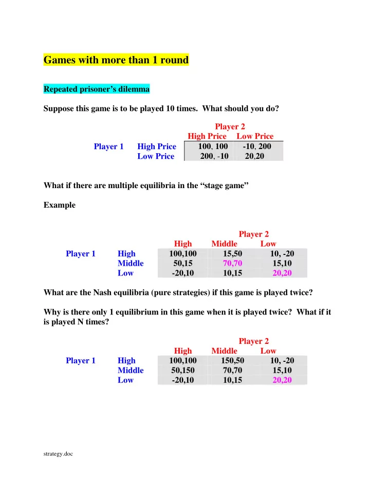
Repeated prisoner’s dilemma Suppose this game is to be played 10 times. What should you do? Player 2 High Price Low Price Player 1 High Price 100, 100 -10, 200 Low Price 200, -10 20,20 What if there are multiple equilibria in the “stage game” Example Player 2 High Middle Low Player 1 High 100,100 15,50 10, -20 Middle 50,15 70,70 15,10 Low

• 20,10

10,15 20,20 What are the Nash equilibria (pure strategies) if this game is played twice? Why is there only 1 equilibrium in this game when it is played twice? What if it is played N times? Player 2 High Middle Low Player 1 High 100,100 150,50 10, -20 Middle 50,150 70,70 15,10 Low

• 20,10

10,15 20,20

1

Games without a definite end-date

Consider a prisoner’s dilemma game. There are two firms. In each period, t=1,2.... each sets either a High or Low price. Profits in the period are as follows. firm 2 High Low firm 1 High 5,5 0,9 Low 9,0 2,2 Table 12: Prisoners Dilemma As we have seen, if there are only a finite number of periods, the unique strategic equilibrium is to choose Low in the last period, hence Low in the second last period, hence ........ Low in the first period. But what if there is no end-date? Instead, let us assume that the game goes on forever. Suppose that both firms in fact choose to cooperate by setting the High price. The stream of payoffs is then as depicted in Figure 1.

6 4 5 3 2 1 payoff period 5 5 5 5 5 5 Figure 1: Stream of payoffs from continuing to choose High

If firm 2 starts out in this way, can firm 1 do better? This depends not only on firm 1’s immediate payoff, but also on what firm 2 will do if firm 1 should choose to play non-cooperatively (to “cheat”) in the first period. One possibility is that firm 2 will respond by never again trusting firm 1 and hence choosing the Low price. If this is the case, firm 1’s payoff stream is as depicted in Figure 2.

6 4 5 3 2 1 payoff period 2 9 Figure 2: Stream of payoffs from choosing Low 2 2 2 2

2

To compute the present value of this strategy, we let V be the present value of all payoffs following period 1, that is, to the right of the first dotted vertical line. Then the present value of all the payoffs is 9+V. Now move to the second dotted line just after period 2. Looking ahead, the infinite stream is exactly the same as it was after period 1. Thus it also has a value of V when discounted to just after period 2. Adding in the period 2 payoff, the value of the stream discounted to period 2 is 2+V. Then if we discount this stream back to period 1, the present value is (2+V)/(1+r), where r is the interest rate per period. But we began by assuming that the present value from just after period 1 is V. Thus V must satisfy:

V V r = + + 2 1

, or after rearranging, V

r = 2 .

Adding in the first period payoff of 9, the present value of not cooperating is

9 2 + r .

We now compare this with the payoff if both firms cooperate. Arguing exactly as above, the present value of the stream discounted to just after period 1 is 5/r. Then adding in the first period payoff, the present value of cooperating is

5 5 + r .

Then cooperating by choosing the High price has a higher payoff if

(5 ) ( ) ( ) + − + = − = − > 5 9 2 3 4 4 3 4 r r r r r

. Thus in this example, it is better to cooperate as long as the period to period interest rate is less than 0.75. But this is not quite the end of the story. Suppose firm 2 indicates that it will play in the way described above. That is, it will “trust” initially but if it is ever crossed, will never trust again. Is this threat credible? To answer this question we must ask whether the threat is an equilibrium strategy of the game continuing after period 1. Suppose firm 1 chooses Low in the first period. If firm 1 believes that firm 2 will carry out the threat, firm 1’s best response is to play Low. But with firm 1 playing Low, firm 2’s best response is also to play Low. Thus Low is an equilibrium strategy

• f the continuing game. That is, the threat is credible.

RULE: The threatened response to a player that “cheats” is a credible threat if it is a strategic equilibrium strategy of the continuing game.

3

For our example, we have seen that, for r < 0.75 it is a strategic equilibrium for each firm to start out setting a High price and to switch forever, if the other firm even once chooses Low. Now let us look at the prisoner’s dilemma game more generally. Each firm can get a payoff of g, the good payoff, or b the bad payoff. Moreover, if one tries to be good while the other deviates for a short-run gain, the latter gets d, while the former gets s. firm 2 High Low firm 1 High g,g s,d Low d,s b,b Table 13: General 2x2 Prisoners Dilemma Arguing exactly as above, the payoff from trying to steal the market is b d r + while the payoff from cooperating is g g r + . Thus cooperation is the preferred strategy if ( ) ( ) ( ) ( ) g b g b d g g b g d d g r r r r r d g − − − + − + = − − = − > − For a prisoner’s dilemma game we require d > g > b > s thus the first term in the final parentheses is positive. It follows that as long as the interest rate is sufficiently low, cooperation is possible in any infinitely repeated prisoner’s dilemma game1.

1 My Scottish ancestral clan seems to have understood this principle well. The clan motto is “Never forget a friend,

never forgive an enemy!”

4

We next consider a slightly more complicated situation where there are several alternatives to pricing non-cooperatively. For example, suppose, as in Table 14 that the two firms are considering three possible pricing strategies. As before, it is readily confirmed that both pricing Low is an equilibrium. Moreover, just as before, there is a cooperative equilibrium in which any cheating is punished forever. firm 2 High Middle Low High 7,3 5,6 2,7 firm 1 Middle 10,1 6,2 3,3 Low 11,-2 7,-1 4,0 Table 14: Prisoners Dilemma with three alternatives But these are not the only two equilibria. Firm 1 might argue that, because it is more profitable, it should get a better deal from cooperation. It announces a strategy of setting a Middle price and holding there as long as firm 2 keeps its price High. If firm 2 ever chooses a price other than High, firm 1 will switch to Low forever. It is left to the reader to confirm that this is also a strategic equilibrium.2 RULE: In games without a definite end-date, there are many strategic equilibria. The choice of an equilibrium thus hinges on the ability of the parties to agree on which pair of equilibrium strategies they will play. Whenever there are multiple equilibria, the power of the theory is greatly weakened unless there is some other reason why one equilibrium is more plausible than another.

2 There is another equilibrium in which firm 2 chooses Middle initially and firm 1 chooses High. Does this seem as

plausible? Why, or why not?

5

Cournot Duopoly Choosing output levels firm 2 Low Middle High Low 72,72 60,80 54,81 firm 1 Middle 80,60 64,64 56,63 High 11,-2 63,56 64,64 For what interest rates does it pay to cooperate? Consider the following example

1 2

30 , ( ) 6

i i

p q q C q q = − − =

6

Cooperation with an uncertain end-date As an alternative to the above model, suppose that the game will end at some point but neither player knows exactly when this will be. Perhaps at some point a large firm will enter the market and eliminate the profit of both players. We model this by assuming that, if the game gets to period t there is a probability p that the game will end and a probability 1-p that the game will continue to period t+1. Suppose that once again firm 2 threatens to never cooperate again if firm 1 deviates even once. Let c be the payoff if both “cooperate” and let n be the Nash equilibrium payoff in the stage game. Finally let d > c be the biggest one period payoff if someone “defects.” Reducing what might be a much larger game to its essential elements, we have the following payoff matrix. firm 2 Left Right firm 1 Top c,c s,d Bottom d,s n,n The payoff tree for player 1 if he deviates is as depicted below.

4 3 2 1 period Figure 3: Payoff tree from choosing Low

n n n d

p p p p 1-p 1-p 1-p 1-p

7

Let V be the present expected value of the stream of benefits after period 1. Arguing as before, if we move forward to period 2, the discounted expected value of the stream from then on must be n+ V. Discounting back to period 1, this stream has period 1 present value of 1 n V r + + . This outcome occurs with probability 1-p. With probability p the game ends and the profit is zero. Then (1 )( ) 1 n V V p r + = − + . Rearranging, (1 ) (1 ) (1 ) V r V p n p + − − = − hence 1 ( )2 p V r p − = + Suppose for simplicity that the interest rate is zero. The expected present value of the entire tree is thus 1 ( 1) d n p + − . Arguing as above, if both players cooperate, the expected present value is 1 ( 1) c c p + − The net gain to cooperating is therefore 1 ( 1)( ) ( ) c n d c p − − − − and this is positive as long as c n p d n − < − . Thus as long as the probability of the current round being the last is not too high, cooperation yields a higher payoff than one short-run gain followed by a low payoff thereafter. Once again this is not the end of the story since we must check that the planned response to “cheating” is a strategic equilibrium of the continuing game. It is left to the reader to check that the argument made in the previous section holds here as well.

8

Bargaining Consider some opportunity which will yield a potential partnership a total profit of $V per year for Y years. (For simplicity we will ignore discounting.) The two potential partners, Alex and Bev, have to first reach agreement on the share of the profit each will receive. Alex might start out by demanding (say) 70% of the gain and saying that if Bev does not immediately agree, she will ever-after raise her demand to 80%. If Bev believes this she has a best reply of “Accept any offer of at least 70%”. And if Bev has this strategy, Alex’s offer is a best response to Bev. Of course Bev might start out with her own “outrageous” offer - -demanding (say a 90% share and indicating that she will refuse to budge. Again we have a strategic equilibrium. It appears, therefore that game theory produces an embarrassment of riches - -almost any outcome can be a strategic equilibrium. However, if each round of bargaining takes time, and hence there is a cost of delay, a very different conclusion emerges. Let there be T periods with one round of bargaining per period. Let v be the profit per period (so that vT = VY). Bargaining takes the form of alternating offers and counteroffers. As in any alternating move game, we look forward to the end of the game and figure

• ut what players would do if they get to that point. We then work backwards.

Rounds Offer by total profit offer payoffs if share to go rejected 1 Alex v (v,0) (0,0) (100,0) 2 Bev 2v (v,v) (v,0) (50,50) 3 Alex 3v (2v,v) (v,v) (67,33) 4 Bev 4v (2v,2v) (2v,v) (50,50) ................. 11 Alex 11v (6v,5v) (5v,5v) (55,45)

9

It is readily checked that with an even number of rounds to go, the offer is always a 50:50 split. Moreover, as the number of rounds grows, the share offered in the odd numbered rounds approaches the equal split as well. Thus if the time between rounds is fairly short and thus the potential number of rounds is large, the advantage to moving last is very small and the two parties agree to an equal share. Outside alternative Suppose Alex can earn v A per round in some alternative activity if in each period where agreement is not reached, while Bev can earn vB., where both are less than

v / 2 . How would this affect the discussion above?

Hint: In each period there is a potential surplus of

A B

x v v v = − − . In the last period Alex can claim all of this surplus since if Bev rejects she earns

B

v . Costly delay Another cost of bargaining is the cost of time. That is, if you agree to a 50:50 split

• f $1 million a period from now this is only worth

1 1 r δ = + million today. Suppose that if agreement is reached at time t the value of the agreement discounted to that period will be v. Suppose Alex moves at t=1 first and Bev at t=2. Let

A

v be the present value of Alex at t=3 given the equilibrium bargaining strategies and let

B

v be the present value to Bev.

10

Since the future at t=3 is identical to the future at t=1 the equilibrium payoff at t=1 must be the same. Thus ( )

A A

v v v v δ δ = − − Rearranging,

2

1 1 1 (1 )(1 ) 1

A

v v v v δ δ δ δ δ δ − − = = = − − + + Since the values add up to 1, 1 1 1

B

v v v δ δ δ = − = + + . Thus if the time between rounds is short so the discount factor is close to 1, the shares are approximately equal.

t=3

B

v

A

v

Bev Alex t=2 t=1

A

v v δ − ( )

A

v v δ δ − ( )

A

v v v δ δ − −

A

v δ

11

War of Attrition

Payoff to the victor V Cost per period (litigation) c Seek a symmetric equilibrium in which exit occurs each round with probability p. If both exit each has an equal chance of winning. Suppose that firm 2 adopts this strategy. If firm 1 exits immediately its expected payoff is

1 1 2 2

Pr{opponent exits immediately} V pV = . If firm 1 plans to exit after 1 period it incurs round 1 litigation costs. Its expected payoff is

1 2

Pr{opponent exits immediately} Pr{opponent exits in round 2}( ) c V V − + +

1 2

(1 ) c pV p p V = − + + − . For a mixed strategy equilibrium firm 1 must be indifferent.

1 1 2 2

(1 ) p V c pV p p V = − + + − Rearranging,

2

2 2 c p p V − + = − Hence

2 2

2 (1 ) 1 2 1 c p p p V − = − + = − . Therefore 2 1 1 c p V = − − . The larger the ratio of c to V the larger the probability of quitting and hence the less wasteful battling.

12

c/v p 0.2 0.23 0.15 0.16 0.1 0.11 0.05 0.05 0.01 0.01