G odel Logic: from Natural Deduction to Parallel Computation - - PDF document

G¨

• del Logic: from Natural Deduction to Parallel

Computation

Federico Aschieri

Institute of Discrete Mathematics and Geometry TU Wien, Austria

Agata Ciabattoni

Theory and Logic Group TU Wien, Austria

Francesco A. Genco

Theory and Logic Group TU Wien, Austria

Abstract—Propositional G¨

• del

logic G extends intuition- istic logic with the non-constructive principle

• f

linearity (A → B) ∨ (B → A). We introduce a Curry–Howard correspon- dence for G and show that a simple natural deduction calculus can be used as a typing system. The resulting functional language extends the simply typed λ-calculus via a synchronous commu- nication mechanism between parallel processes, which increases its expressive power. The normalization proof employs original termination arguments and proof transformations implementing forms of code mobility. Our results provide a computational interpretation of G, thus proving A. Avron’s 1991 thesis.

• I. INTRODUCTION

Logical proofs are static. Computations are dynamic. It is a striking discovery that the two coincide: formulas correspond to types in a programming language, logical proofs to programs of the corresponding types and removing detours from proofs to evaluation of programs. This correspondence, known as Curry– Howard isomorphism, was first discovered for constructive proofs, and in particular for intuitionistic natural deduction and typed λ-calculus [20] and later extended to classical proofs, despite their use of non-constructive principles, such as the excluded middle [18], [2] or reductio ad absurdum [17], [30]. Nowadays various different logics (linear [8], modal [28] ...) have been related to many different notions of computation; the list is long, and we refer the reader to [34]. G¨

• del logic, Avron’s conjecture and previous attempts

Twenty-five years have gone by since Avron conjectured in [3] that G¨

• del logic G [16] – one of the most useful and inter-

esting logics intermediate between intuitionistic and classical logic – might provide a basis for parallel λ-calculi. Despite the interest of the conjecture and despite various attempts, no Curry–Howard correspondence has so far been provided for G. The main obstacle has been the lack of an adequate natural deduction calculus. Well designed natural deduction inferences can indeed be naturally interpreted as program instructions, in particular as typed λ-terms. Normalization [32], which corresponds to the execution of the resulting programs, can then be used to obtain proofs only containing formulas that are subformulas of some of the hypotheses or of the conclusion. However the problem of finding a natural deduction for G with this property, called analyticity, looked hopeless for decades.

Supported by FWF: grants M 1930–N35, Y544-N2, and W1255-N23.

All approaches explored so far to provide a precise formal- ization of G as a logic for parallelism, either sacrificed analyt- icity [1] or tried to devise forms of natural deduction whose structures mirror hypersequents – which are sequents operating in parallel [4]. Hypersequents were indeed successfully used in [3] to define an analytic calculus for G and were intuitively connected to parallel computations: the key rule introduced by Avron to capture the linearity axiom – called communication – enables sequents to exchange their information and hence to “communicate”. The first analytic natural deduction calculus proposed for G [5] uses indeed parallel intuitionistic derivations joined together by the hypersequent separator. Normalization is obtained there only by translation into Avron’s calculus: no reduction rules for deductions and no corresponding λ- calculus were provided. The former task was carried out in [6], that contains a propositional hyper natural deduction with a normalization procedure. The definition of a corresponding λ-calculus and Curry–Howard correspondence are left as an

• pen problem, which might have a complex solution due to

the elaborated structure of hyper deductions. Another attempt along the “hyper line” has been made in [19]. However, not

• nly the proposed proof system is not shown to be analytic, but

the associated λ-calculus is not a Curry–Howard isomorphism: the computation rules of the λ-calculus are not related to proof transformations, i.e. Subject Reduction does not hold. λG: Our Curry–Howard Interpretation of G¨

• del Logic

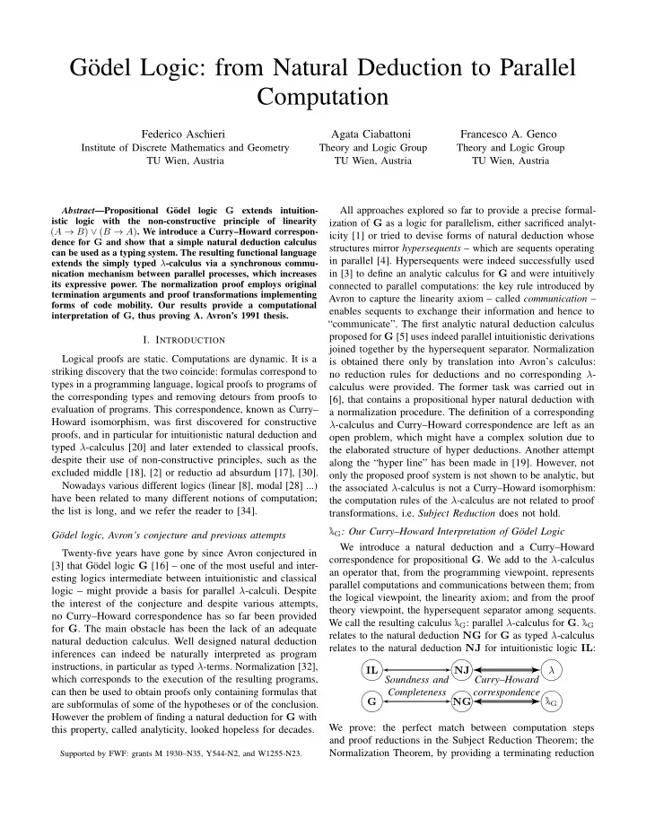
We introduce a natural deduction and a Curry–Howard correspondence for propositional G. We add to the λ-calculus an operator that, from the programming viewpoint, represents parallel computations and communications between them; from the logical viewpoint, the linearity axiom; and from the proof theory viewpoint, the hypersequent separator among sequents. We call the resulting calculus λG: parallel λ-calculus for G. λG relates to the natural deduction NG for G as typed λ-calculus relates to the natural deduction NJ for intuitionistic logic IL: IL NJ λ G NG λG Soundness and Completeness Curry–Howard correspondence We prove: the perfect match between computation steps and proof reductions in the Subject Reduction Theorem; the Normalization Theorem, by providing a terminating reduction

strategy for λG; the Subformula Property, as corollary. The expressive power of λG is illustrated through examples of programs and connections with the π-calculus [26], [33]. The natural deduction calculus NG that we use as type sys- tem for λG is particularly simple: it extends NJ with the (com) rule (its typed version is displayed below), which was first considered in [24] to define a natural deduction calculus for G, but with no normalization procedure. The calculus NG follows the basic principle of natural deduction that new axioms require new computational reductions; this contrasts with the basic principle of sequent calculus employed in the “hyper approach”, that new axioms require new deduction structures. Hence we keep the calculus simple and deal with the complexity of the hypersequent structure at the operational side. Consequently, the programs corresponding to NG proofs maintain the syntactical simplicity of λ-calculus. The normalization procedure for NG extends Prawitz’s method with ideas inspired by hypersequent cut-elimination, by normalization in classical logic [2] and by the embedding in [10] between hypersequents and systems of rules [29]; the latter shows that (com) reformulates Avron’s communication rule. The inference rules of NG are decorated with λG-terms, so that we can directly read proofs as typed programs. The decoration of the NJ inferences is standard and the typed version of (com) is [aA→B : A → B] . . . . u : C [aB→A : B → A] . . . . v : C u a v : C com Inspired by [1], we use the variable a to represent a private communication channel between the processes u and v. The computational reductions associated to a – cross reductions – enjoy a natural interpretation in terms of higher-order process passing, a feature which is not directly rendered through communication by reference [31] and is also present in higher-

• rder π-calculus [33]. Nonetheless cross reductions handle

more subtle migration issues. In particular, a cross reduction can be activated whenever a communication channel a is ready to transfer information between two parallel processes: C[a u] a D[a v] Here C is a process containing a fragment of code u, and D is a process containing a fragment of code v. Moreover, C has to send u through the channel a to D, which in turn needs to send v through a to C. In general we cannot simply send the programs u and v: some resources in the computational environment that are used by u and v may become inaccessible from the new locations [14]. Cross reductions solve the problem by exchanging the location of u and v and creating a new communication channel for their resources. Technically, the channel takes care of closures – the contexts containing the definitions of the variables used in a function’s body [23]. Several programming languages such as JavaScript, Ruby or Swift provide mechanisms to support and handle closures. In

• ur case, they are the basis of a process migration mechanism

handling the bindings between code fragments and their computational environments. Cross reductions also improve the efficiency of programs by facilitating partial evaluation of

• pen processes (see Example VII.4).
• II. PRELIMINARIES ON G ¨

ODEL LOGIC

Also known as G¨

• del–Dummett logic [12], G¨
• del logic G

naturally turns up in a number of different contexts; among them, due to the natural interpretation of its connectives as functions over the real interval [0, 1], G is one of the best known ‘fuzzy logics’, e.g. [25]. Although propositional G is obtained by adding the linearity axiom (lin) (A → B) ∨ (B → A) to any proof calculus for intuitionistic logic, analytic calculi for G have only been defined in formalisms extending the sequent calculus. Among them, arguably, the hypersequent calculus in [3] is the most successful one, see, e.g., [25]. In general a hypersequent calcu- lus is defined by incorporating a sequent calculus (Gentzen’s LJ, in case of G) as a sub-calculus and allowing sequents to live in the context of finite multisets of sequents. Definition II.1. A hypersequent is a multiset of sequents, written as Γ1 ⇒ Π1 | . . . | Γn ⇒ Πn where, for all i = 1, . . . n, Γi ⇒ Πi is an ordinary sequent. The symbol “|” is a meta-level disjunction; this is reflected by the presence in the calculus of the external structural rules

• f weakening and contraction, operating on whole sequents,

rather than on formulas. The hypersequent design opens the possibility of defining new rules that allow the “exchange of information” between different sequents. It is this type of rules which increases the expressive power of hypersequent calculi compared to sequent calculi. The additional rule employed in Avron’s calculus for G [3] is the so called communication rule, below presented in a slightly reformulated version (as usual G stands for a possibly empty hypersequent):

G | Γ1, B ⇒ C G | Γ2, A ⇒ D G | Γ1, A ⇒ C | Γ2, B ⇒ D

• III. NATURAL DEDUCTION

The very first step in the design of a Curry–Howard corre- spondence is to lay a solid logical foundation. No architectural mistake is allowed at this stage: the natural deduction must be structurally simple and the reduction rules as elementary as possible. We present such a natural deduction system NG for G¨

• del logic. NG extends Gentzen’s propositional natural

deduction NJ (see [32]) with a rule accounting for axiom (lin). We describe the reduction rules for transforming every NG deduction into an analytic one and present the ideas behind the Normalization Theorem, which is proved in the λ-calculus framework in Section VI. NG is the natural deduction version of the sequent calculus with systems of rules in [29]; the latter embeds (into) Avron’s hypersequent calculus for G. Indeed [10] introduces a mapping from (and into) derivations in Avron’s calculus into (and from)

derivations in the LJ sequent calculus for intuitionistic logic with the addition of the system of rules

B, Γ1 ⇒ C A, Γ1 ⇒ C (com1) . . . . Γ ⇒ Π A, Γ2 ⇒ D B, Γ2 ⇒ D (com2) . . . . Γ ⇒ Π Γ ⇒ Π (comend)

where (com1), (com2) can only be applied (possibly many times) above respectively the left and right premise of (comend). The above system, that reformulates Avron’s communication rule, immediately translates into the natural deduction rule below, whose addition to NJ leads to a natural deduction calculus for G

. . . B A coml . . . . C . . . A B comr . . . . C C com

Not all the branches of a derivation containing the above rule are NJ derivations. To avoid that, and to keep the proof of the Subformula Property (Theorem V.4) as simple as possible, we use the equivalent rule below, first considered in [24]. Definition III.1 (NG). The natural deduction calculus NG extends NJ with the (com) rule: [A → B] . . . . C [B → A] . . . . C C com Let ⊢NG and ⊢G indicate the derivability relations in NG and in NJ + (lin), respectively. Theorem III.1 (Soundness and Completeness). For any set Π

• f formulas and formula A, Π ⊢NG A if and only if Π ⊢G A.
• Proof. (⇒) Applications of (com) can be simulated by ∨

eliminations having as major premiss an instance of (lin). (⇐) Easily follows by the following derivation: [A → B]1 (A → B) ∨ (B → A) [B → A]1 (A → B) ∨ (B → A) (A → B) ∨ (B → A) com1

• Notation. To shorten derivations henceforth we will use

A coml B B comr A as abbreviations for [A → B] A B [B → A] B A respectively, and call them communication inferences. As usual, we will use ¬A and ⊤ as shorthand for A → ⊥ and ⊥ → ⊥. Moreover, we exploit the equivalence of A ∨ B and ((A → B) → B) ∧ ((B → A) → A) in G (see [12]) and treat ∨ as a defined connective.

• A. Reduction Rules and Normalization

A normal deduction in NG should have two essential features: every intuitionistic Prawitz-style reduction should have been carried out and the Subformula Property should

• hold. Due to the (com) rule, the former is not always enough

to guarantee the latter. Here we present the main ideas behind the normalization procedure for NG and the needed reduction

• rules. The computational interpretation of the rules will be

carried out through the λG calculus in Section IV. The main steps of the normalization procedure are as follows:

• We permute down all applications of (com).

The resulting deduction – we call it in parallel form – consists of purely intuitionistic subderivations joined together by consecutive (com) inferences occurring immediately above the root. This transformation is a key tool in the embedding between hypersequents and systems of rules [10]. The needed reductions are instances of Prawitz-style permutations for ∨

• elimination. Their list can be obtained by translating into natural

deduction the permutations in Fig. 1. Once obtained a parallel form, we interleave the following two steps.

• We apply the standard intuitionistic reductions ([32]) to

the parallel branches of the derivation. This way we normalize each single intuitionistic derivation, and this can be done in parallel. The resulting derivation, however, need not satisfy yet the Subformula Property. Intuitively, the problem is that communications may discharge hypotheses that have nothing to do with their conclusion.

• We apply specific reductions to replace the (com) appli-

cations that violate the Subformula Property. These reductions – called cross reductions – account for the hypersequent cut-elimination. They allow to get rid of the new detours that appear in configurations like the one below on the left. To remove these detours, a first idea would be to simultaneously move the deduction D1 to the right and D2 to the left thus obtaining the derivation below right: D1 A B coml . . . . C D2 B A comr . . . . C C com D2 B . . . . C D1 A . . . . C C In fact, in the context of Krivine’s realizability, Danos and Krivine [9] studied the linearity axiom as a theorem of classical logic and discovered that its realizers implement a restricted version of this transformation. Their transformation does not lead however to the subformula property for NG. The unrestricted transformation above, on the other hand, cannot work; indeed D1 might contain the hypothesis A → B and hence it cannot be moved on the right. Even worse, D1 may depend on hypotheses that are locally opened, but discharged below B but above C. Again, it is not possible to move D1 on the right as naively thought, otherwise new global hypotheses would be created.

We overcome these barriers by our cross reductions. Let us highlight Γ and ∆, the hypotheses of D1 and D2 that are respectively discharged below B and A but above the application of (com). Assume moreover, that A → B does not occur in D1 and B → A does not occur in D2 as hypotheses discharged by (com). A cross reduction transforms the deduction below left into the deduction below right (if (com) in the original proof discharges in each branch exactly

• ne occurrence of the hypotheses, and Γ and ∆ are formulas)

Γ D1 A B coml . . . . C ∆ D2 B A comr . . . . C C com ∆ Γ coml D1 A . . . . C Γ ∆ comr D2 B . . . . C C com and into the following deduction, in the general case Γ D1 A B com1

l

. . . . C ∆ Γ com3

l

D1 A . . . . C C com1 Γ ∆ com3

r

D2 B . . . . C ∆ D2 B A com2

r

. . . . C C com2 C com3 where the double bar notation stands for an application of (com) between sets of hypotheses Γ and ∆, which means to prove from Γ the conjunction of the formulas of Γ, then to prove the conjunction of the formulas of ∆ by means of a communication inference and finally obtain each formula of ∆ by a series of ∧ eliminations, and vice versa. Mindless applications of the cross reductions might lead to dangerous loops, see e.g. Example IV.2. To avoid them we will allow cross reductions to be performed only when the proof is not analytic. Thanks to this and to other restrictions, we will prove termination and thus the Normalization Theorem.

• IV. THE λG-CALCULUS

We introduce λG, our parallel λ-calculus for G. λG extends the standard Curry–Howard correspondence [34] for intuition- istic natural deduction with a parallel operator that interprets the inference for the linearity axiom. We describe λG-terms and their computational behavior, proving as main result of the section the Subject Reduction Theorem, stating that the reduction rules preserve the type.

Axioms xA : A Conjunction u : A t : B u, t : A ∧ B u : A ∧ B u π0 : A u : A ∧ B u π1 : B Implication [xA : A] . . . . u : B λxAu : A → B t : A → B u : A tu : B Linearity Axiom [aA→B : A → B] . . . . u : C [aB→A : B → A] . . . . v : C u a v : C Ex Falso Quodlibet Γ ⊢ u : ⊥ Γ ⊢ efqP (u) : P with P atomic, P = ⊥.

The table above defines a type assignment for λG-terms, called proof terms and denoted by t, u, v . . . , which is isomorphic to NG. The typing rules for axioms, implication, conjunction and ex-falso-quodlibet are standard and give rise to the simply typed λ-calculus, while parallelism is introduced by the rule for the linearity axiom. Proof terms may contain variables xA

0 , xA 1 , xA 2 , . . . of type

A for every formula A; these variables are denoted as xA, yA, zA, . . . , aA, bA, cA and whenever the type is not important simply as x, y, z, . . . , a, b. For clarity, the variables introduced by the (com) rule will be often denoted with letters a, b, c, . . ., but they are not in a syntactic category apart. A variable xA that

• ccurs in a term of the form λxAu is called λ-variable and a

variable a that occurs in a term u a v is called communication variable and represents a private communication channel between the parallel processes u and v. The free and bound variables of a proof term are defined as usual and for the new term u a v, all the free occurrences of a in u and v are bound in u a v. In the following we assume the standard renaming rules and alpha equivalences that are used to avoid capture of variables in the reduction rules.

• Notation. The connective → associates to the right and by

t1, t2, . . . , tn we denote the term t1, t2, . . . tn−1, tn . . . and by πi, for i = 0, . . . , n, the sequence of projections π1 . . . π1π0 selecting the (i + 1)th element of the sequence. Therefore, for every formula sequence A1, . . . , An the expres- sion A1 ∧ . . . ∧ An denotes (A1 ∧ (A2 ∧ . . . (An−1 ∧ An) . . . ))

• r ⊤ if n = 0.

Often, when Γ = x1 : A1, . . . , xn : An and the list x1, . . . , xn includes all the free variables of a proof term t : A, we shall write Γ ⊢ t : A. From the logical point of view, t represents a natural deduction of A from the hypotheses A1, . . . , An. We shall write G ⊢ t : A whenever ⊢ t : A, and the notation means provability of A in propositional G¨

• del
• logic. If the symbol does not occur in it, then t is a simply

typed λ-term representing an intuitionistic deduction. We define as usual the notion of context C[ ] as the part

• f a proof term that surrounds a hole, represented by some

fixed variable. In the expression C[u] we denote a particular

• ccurrence of a subterm u in the whole term C[u]. We shall

just need those particularly simple contexts which happen to be simply typed λ-terms. Definition IV.1 (Simple Contexts). A simple context C[ ] is a simply typed λ-term with some fixed variable [] occurring exactly once. For any proof term u of the same type of [], C[u] denotes the term obtained replacing [] with u in C[ ], without renaming of any bound variable. As an example, the expression C[ ] := λx z ([]) is a simple context and the term λx z (x z) can be written as C[xz].

We define below the notion of stack, corresponding to Krivine stack [21] and known as continuation because it embodies a series of tasks that wait to be carried out. A stack represents, from the logical perspective, a series of elimination rules; from the λ-calculus perspective, a series

• f either operations or arguments.

Definition IV.2 (Stack). A stack is a sequence σ = σ1σ2 . . . σn such that for every 1 ≤ i ≤ n, exactly one

• f the following holds: either σi = t, with t proof term or

σi = πj, with j ∈ {0, 1}. We will denote the empty sequence with ǫ and with ξ, ξ′, . . . the stacks of length 1. If t is a proof term, as usual t σ denotes the term (((t σ1) σ2) . . . σn). We define now the notion of strong subformula, which is essential for defining the reduction rules of the λG-calculus and for proving Normalization. The technical motivations will become clear in Sections V and VI, but the intuition is that the new types created by cross reductions must be always strong subformulas of already existing types. To define the concept

• f strong subformula we also need the following definition.

Definition IV.3 (Prime Formulas and Factors [22]). A formula is said to be prime if it is not a conjunction. Every formula is a conjunction of prime formulas, called prime factors. Definition IV.4 (Strong Subformula). B is said to be a strong subformula of a formula A, if B is a proper subformula of some prime proper subformula of A. Note that in the present context, prime formulas are either atomic formulas or arrow formulas, so a strong subformula of A must be actually a proper subformula of an arrow proper subformula of A. The following characterization of the strong subformula relation will be often used. Proposition IV.1 (Characterization of Strong Subformulas). Suppose B is any strong subformula of A. Then:

• If A = A1 ∧ . . . ∧ An, with n > 0 and A1, . . . , An are

prime, then B is a proper subformula of one among A1, . . . , An.

• If A = C → D, then B is a proper subformula of a prime

factor of C or D. Proof. Simple considerations on the structure of A. Definition IV.5 (Multiple Substitution). Let u be a proof term, x = xA0

0 , . . . , xAn n

a sequence of variables and v : A0∧. . .∧An. The substitution uv/x := u[v π0/xA0 . . . v πn/xAn

n ] replaces

each variable xAi

i

• f any term u with the ith projection of v.

We now seek a measure for determining how complex the communication channel a of a term u a v is. Logic will be

• ur guide. First, it makes sense to consider the types B, C

such that a occurs with type B → C in u and thus with type C → B in v. Moreover, assume u a v has type A and its free variables are xA1

1 , . . . , xAn n . The Subformula Property tells us

that, no matter what our notion of computation will turn out to be, when the computation is done, no object of type more complex than the types of the inputs and the output should

• appear. Hence, if the prime factors of the types B and C are

not subformulas of A1, . . . , An, A, then these prime factors should be taken into account in the complexity measure we are looking for. The actual definition is the following. Definition IV.6 (Communication Complexity). Let u a v : A a proof term with free variables xA1

1 , . . . , xAn n . Assume that

aB→C occurs in u and thus aC→B in v.

• The pair B, C is called the communication kind of a.
• The communication complexity of a is the maximum

among 0 and the numbers of symbols of the prime factors

• f B or C that are neither proper subformulas of A nor

strong subformulas of one among A1, . . . , An. We explain now the basic reduction rules for the proof terms

• f λG, which are given in Figure 1. As usual, we also have the

reduction scheme: E[t] → E[u], whenever t → u and for any context E. With →∗ we shall denote the reflexive and transitive closure of the one-step reduction →. Intuitionistic Reductions. These are the very familiar com- putational rules for the simply typed λ-calculus, representing the operations of applying a function and taking a component

• f a pair [15]. From the logical point of view, they are the

standard Prawitz reductions [32] for NJ. Cross Reductions. The reduction rules for (com) model a communication mechanism between parallel processes. In

• rder to apply a cross reduction to a term

C[a u] a D[a v] several conditions have to be met. These conditions are both natural and needed for the termination of computations. First, we require the communication complexity of a to be greater than 0; again, this is a warning that the Subformula Property does not hold. Here we use a logical property as a computational criterion for answering the question: when should computation stop? An answer is crucial here, because, as shown in Example IV.2, unrestricted cross reductions do not always terminate. In λ-calculi the Subformula Property fares pretty well as a stopping criterion. In a sense, it detects all the essential operations that really have to be done. For example, in simply typed λ-calculus, a closed term that has the Subformula Property must be a value, that is, of the form λx u, or u, v. Indeed a closed term which is a not a value, must be of the form h σ, for some stack σ (see Definition IV.2), where h is a redex (λy u)t or u, v πi; but (λy u) and u, v would have a more complex type than the type of the whole term, contradicting the Subformula Property. Second, we require C[a u], D[a v] to be normal simply typed λ-

• terms. Simply typed λ-terms, because they are easier to execute

in parallel; normal, because we want their computations to go

• n until they are really stuck and communication is unavoidable.

Third, we require the variable a to be as rightmost as possible and that is needed for logical soundness: how could otherwise the term u be moved to the right, e.g., if it contains a? Assuming that all the conditions above are satisfied, we can now start to explain the cross reduction

C[a u] a D[a v] → (D[ubz/y] a C[a u]) b (C[vby/z] a D[a v])

Here, the communication channel a has been activated, because the processes C and D are synchronized and ready to transfer respectively u and v. The parallel operator a let the two

• ccurrences of a communicate: the term u travels to the right

in order to replace a v and v travels to the left in order to replace a u. If u and v were data, like numbers or constants, everything would be simple and they could be sent as they are; but in general, this is not possible. The problem is that the free variables y of u which are bound in C[a u] by some λ cannot be permitted to become free; otherwise, the connection between the binders λ y and the occurrences of the variables y would be lost and they could be no more replaced by actual values when the inputs for the λ y are available. Symmetrically, the variables z cannot become free. For example, we could have u = u′ y and v = v′ z and

C[a u] = w1 (λy a (u′ y)) D[a v] = w2 (λz a (v′ z))

and the transformation

w1 (λy a (u′ y)) a w2 (λz a (v′ z)) → w1 (λy v′ z) a w2 (λz u′ y) would just be wrong: the term v′ z

will never get back actual values for the variables z when they will become available. These issues are typical of process migration, and can be solved by the concepts of code mobility [14] and closure [23]. Informally, code mobility is defined as the capability to dynamically change the bindings between code fragments and the locations where they are executed. Indeed, in order to be executed, a piece of code needs a computational environment and its resources, like data, program counters or global variables. In our case the contexts C[ ] and D[ ] are the computational environments or closures of the processes u and v and the variables y, z are the resources they need. Now, moving a process outside its environment always requires extreme care: the bindings between a process and the environment resources must be preserved. This is the task of the migration mechanisms, which allow a migrating process to resume correctly its execution in the new location. Our migration mechanism creates a new communication channel b between the programs that have been exchanged. Here we see the code fragments u and v, with their original bindings to the global variables y and z. The change of variables ubz/y and vby/z has the effect of reconnecting u and v to their old inputs: In this way, when they will become available, the data y will be sent to u and the data z will be sent to v through the channel

• b. Note that in the result of the cross reduction the processes

C[a u] and D[a v] are cloned, because their code fragments can be needed again. Thus a behaves as a replicated input and replicated output channel. E.g., in [8], replicated input is coded by the bang operator of linear logic: xy.Q | !x(z).P → Q | P[y/z] | !x(z).P With symmetrical message passing and a “!” also in front of xy.Q, one would obtain a version of our cross reduction. Finally, as detailed in Ex. VII.2, whenever u and v are closed terms the cross reduction is simpler and only maintains the first two of the four processes produced in the general case. Example IV.1 (a in λG and | in the π-calculus). A private channel u a v is rendered in the π-calculus [26], [33] by the restriction operator ν, as νa (u | v). Recall that the π-calculus term u | v represents two processes that run in parallel. The corresponding λG term e, u e e, v is defined using a fresh channel e with communication kind A, A. As no cross reduction

• utside u and v can be applied, the whole term reduces neither

to e, u nor to e, v, so that u and v can run in parallel. Example IV.2. Let y and z be bound variables occurring in the normal terms C[a y] and D[a z]. Without the condition on the communication complexity c of a, a loop could be generated:

C[a y] a D[a z] → (D[ybz/y] a C[a y]) b (C[zby/z] a D[a z]) = (D[b z] a C[a y]) b (C[b y] a D[a z]) →∗ D[b z] b C[b y]

In Sec. VI we show that if c > 0, this reduction sequence would

• terminate. What is then happening here? Intuitively, C[a y] and

D[a z] are normal simply typed λ-terms, which forces c = 0. Permutation Reductions. They regulate the interaction be- tween parallel operators and the other computational constructs. The first four reductions are the Prawitz-style permutation rules [32] between parallel operators and eliminations. We also add two other groups of reductions: three permutations between parallel operators and introductions, two permutations between parallel operators themselves. The first group will be needed to rewrite any proof term into a parallel composition of simply typed λ-terms (Proposition V.3). The second group is needed to address the scope extrusion issue of private channels [26]. We point out that a parallel operator a is allowed to commute with other parallel operators only when it is strictly necessary, that is, when the communication complexity of a is greater than 0 and thus signaling a violation of the Subformula Property. Example IV.3 (Scope extrusion (and π-calculus)). As exam- ple of scope extrusion, let us consider the term (v a C[b a]) b w Here the process C[b a] wishes to send the channel a to w along the channel b, but this is not possible being the channel a private. This issue is solved in the π-calculus using the congruence νa(P | Q) | R ≡ νa(P | Q | R), provided that a does not occur in R, condition that can always be satisfied by α-conversion. G¨

• del logic offers and actually forces a different solution,

which is not just permuting w inward but also duplicating it: (v a C[b a]) b w → (v b w) a (C[b a] b w)

After this reduction C[b a] can send a to w. If a does not occur in v, we have a further simplification step: (v b w) a (C[b a] b w) → v a (C[b a] b w)

• btaining associativity of composition as in π-calculus. How-

ever, if b occurs in v, this last reduction step is not possible and we keep both copies of w. It is indeed natural to allow both v and C[b a] to communicate with w. Everything works as expected: the reductions steps in

• Fig. 1 preserve the type at the level of proof terms, i.e., they

correspond to logically sound proof transformations. Indeed Theorem IV.2 (Subject Reduction). If t : A and t → u, then u : A and all the free variables of u appear among those of t.

• Proof. It is enough to prove the theorem for basic reductions:

if t : A and t → u, then u : A. The proof that the intuitionistic reductions and the permutation rules preserve the type is completely standard. Cross reductions require straightforward considerations as well. Indeed suppose

C[a

A→B u] a D[a B→A v]

→ (D[ubD→Cz/y] a C[a

A→B u]) b (C[vbC→Dy/z] a D[a B→A v])

Since y : C := C0 ∧ . . . ∧ Cn and z : D := D0 ∧ . . . ∧ Dm, bD→Cz and bC→Dy are correct terms. Therefore ubD→Cz/y and vbC→Dy/z, by Definition IV.5, are correct as well. The assumptions are that y = yC0

0 , . . . , yCn n

is the sequence of the free variables of u which are bound in C[aA→Bu], z = zD0

0 , . . . , zDm m

is the sequence of the free variables of v which are bound in D[aB→Av], a does not occur neither in u nor in v and b is fresh. Therefore, by construction all the variables z are bound in D[ubD→Cz/y] and all the variables y are bound in C[vbC→Dy/z]. Hence, no new free variable is created. Definition IV.7 (Normal Forms and Normalizable Terms).

• A redex is a term u such that u → v for some v and

basic reduction of Figure 1. A term t is called a normal form or, simply, normal, if there is no t′ such that t → t′. We define NF to be the set of normal λG-terms.

• A

sequence, finite

• r

infinite,

• f

proof terms u1, u2, . . . , un, . . . is said to be a reduction of t, if t = u1, and for all i, ui → ui+1. A proof term u of λG is normalizable if there is a finite reduction of u whose last term is a normal form. Definition IV.8 (Parallel Form). A term t is a parallel form whenever, removing the parentheses, it can be written as t = t1 a1 t2 a2 . . . an tn+1 where each ti, for 1 ≤ i ≤ n + 1, is a simply typed λ-term.

• V. THE SUBFORMULA PROPERTY

We show that normal λG-terms satisfy the important Subfor- mula Property (Theorem V.4). This, in turn, implies that our Curry–Howard correspondence for λG is meaningful from the logical perspective and produces analytic NG proofs. We start by establishing an elementary property of simply typed λ-terms, which will turn out to be crucial for our normalization proof. It ensures that every bound hypothesis appearing in a normal intuitionistic proof is a strong subformula

• f one the premises or a proper subformula of the conclusion.

This property sheds light on the complexity of cross reductions, because it implies that the new formulas introduced by these

• perations are always smaller than the local premises.

Proposition V.1 (Bound Hypothesis Property). Suppose xA1

1 , . . . , xAn n

⊢ t : A t ∈ NF is a simply typed λ-term and z : B a variable occurring bound in t. Then one of the following holds: 1) B is a proper subformula of a prime factor of A. 2) B is a strong subformula of one among A1, . . . , An.

• Proof. By induction on t.

The next proposition says that each occurrence of any hypothesis of a normal intuitionistic proof must be followed by an elimination rule, whenever the hypothesis is neither ⊥ nor a subformula of the conclusion nor a proper subformula

• f some other premise.

Proposition V.2. Let t ∈ NF be a simply typed λ-term and xA1

1 , . . . , xAn n , zB ⊢ t : A

One of the following holds: 1) Every occurrence of zB in t is of the form zB ξ for some proof term or projection ξ. 2) B = ⊥ or B is a subformula of A or a proper subformula

• f one among the formulas A1, . . . , An.
• Proof. Easy structural induction on the term.

Proposition V.3 (Parallel Normal Form Property). If t ∈ NF is a λG-term, then it is in parallel form.

• Proof. Easy structural induction on t using the permutation

reductions. We finally prove the Subformula Property: a normal proof does not contain concepts that do not already appear in the premises or in the conclusion. Theorem V.4 (Subformula Property). Suppose xA1

1 , . . . , xAn n

⊢ t : A and t ∈ NF. Then : 1) For each communication variable a occurring bound in t and with communication kind B, C, the prime factors

• f B and C are proper subformulas of A1, . . . , An, A.

2) The type of any subterm of t which is not a bound commu- nication variable is either a subformula or a conjunction

• f subformulas of the formulas A1, . . . , An, A.
• Proof. We proceed by induction on t. By Proposition V.3

t = t1 a1 t2 a2 . . . an tn+1 and each ti, for 1 ≤ i ≤ n + 1,

Intuitionistic Reductions (λxA u)t → u[t/xA] and u0, u1 πi → ui, for i = 0, 1 Permutation Reductions (u a v)w → uw a vw, if a does not occur free in w w(u a v) → wu a wv, if a does not occur free in w efqP (w1 a w2) → efqP (w1) a efqP (w2) (u a v) πi → u πi a v πi λxA (u a v) → λxA u a λxA v u a v, w → u, w a v, w, if a does not occur free in w w, u a v → w, u a w, v, if a does not occur free in w (u a v) b w → (u b w) a (v b w), if the communication complexity of b is greater than 0 w b (u a v) → (w b u) a (w b v), if the communication complexity of b is greater than 0 Cross Reductions u a v → u, if a does not occur in u and u a v → v, if a does not occur in v C[aA→B u] a D[aB→A v] → (D[ubC→Dz/y] a C[aA→B u]) b (C[vbD→Cy/z] a D[aB→A v]) where C[a u], D[a v] are normal simply typed λ-terms and C, D simple contexts; y is the sequence of the free variables of u which are bound in C[a u]; z is the sequence of the free variables of v which are bound in D[a v]; C and D are the conjunctions of the types of the variables in z and y, respectively; the displayed occurrences of a are the rightmost both in C[a u] and in D[a v]; b is fresh; and the communication complexity of a is greater than 0

• Fig. 1. Basic Reduction Rules for λG

is a simply typed λ-term. We only show the case t = u1 b u2. Let C, D be the communication kind of b, we first show that the communication complexity of b is 0. We reason by contradiction and assume that it is greater than 0. u1 and u2 are either simply typed λ-terms or of the form v c w. The second case is not possible, otherwise a permutation reduction could be applied to t ∈ NF. Thus u1 and u2 are simply typed λ-terms. Since the communication complexity of b is greater than 0, the types C → D and D → C are not subformulas of A1, . . . , An, A. By Prop. V.2, every occurrence of bC→D in u1 is of the form bC→Dv and every occurrence of bD→C in u2 is of the form bD→Cw. Hence, we can write u1 = C[bC→Dv] u2 = D[bD→Cw] where C, D are simple contexts and b is rightmost. Hence a cross reduction of t can be performed, which contradicts the fact that t ∈ NF. Since we have established that the communication complexity of b is 0, the prime factors of C and D must be proper subformulas of A1, . . . , An, A. Now, by induction hypothesis applied to u1 : A and u2 : A, for each communication variable aF →G occurring bound in t, the prime factors of F and G are proper subformulas of the formulas A1, . . . , An, A, C → D, D → C and thus of the formulas A1, . . . , An, A; moreover, the type of any subterm

• f u1 or u2 which is not a communication variable is either a

subformula or a conjunction of subformulas of the formulas A1, . . . , An, C → D, D → C and thus of A1, . . . , An, A. Remark V.1. Our statement of the Subformula Property is slightly different from the usual one. However the latter can be easily recovered using the communication rule (comend)

• f Section III and additional reduction rules. As the resulting

derivations would be isomorphic but more complicated, we prefer the current statement.

• VI. THE NORMALIZATION THEOREM

Our goal is to prove the Normalization Theorem for λG: every proof term of λG reduces in a finite number of steps to a normal form. By Subject Reduction, this implies that NG proofs normalize. We shall define a reduction strategy for terms

• f λG: a recipe for selecting, in any given term, the subterm

to which apply one of our basic reductions. We remark that the permutations between communications have been adopted to simplify the normalization proof, but at the same time, they undermine strong normalization, because they enable silly loops, like in cut-elimination for sequent calculi. Further restrictions of the permutations might be enough to prove strong normalization, but we leave this as an open problem. The idea behind our normalization strategy is to employ a suitable complexity measure for terms u a v and, each time a reduction has to be performed, to choose the term of maximal

• complexity. Since cross reductions can be applied as long as

there is a violation of the Subformula Property, the natural approach is to define the complexity measure as a function of some fixed set of formulas, representing the formulas that can be safely used without violating the Subformula Property. Definition VI.1 (Complexity of Parallel Terms). Let A be a finite set of formulas. The A-complexity of the term u a v is the sequence (c, d, l, o) of natural numbers, where: 1) if the communication kind of a is B, C, then c is the maximum among 0 and the number of symbols of the

prime factors of B or C that are not subformulas of some formula in A; 2) d is the number of occurrences of in u and v; 3) l is the sum of the lengths of the intuitionistic reductions

• f u and v to reach intuitionistic normal form;

4) o is the number of occurrences of a in u and v. For clarity, we define the recursive normalization algorithm that represents the constructive content of the proofs of

• Prop. VI.1 and VI.2, which are used to prove the Normalization
• Theorem. Essentially, our master reduction strategy consists in

iterating the basic reduction relation ≻ defined below, whose goal is to permute the smallest redex u a v of maximal complexity until u and v are simply typed λ-terms, then normalize them and finally apply the cross reductions. Definition VI.2 (Side Reduction Strategy). Let t : A be a term with free variables xA1

1 , . . . , xAn n

and A be the set of the proper subformulas of A and the strong subformulas of the formulas A1, . . . , An. Let u a v the smallest subterm of t, if any, among those of maximal A-complexity and let (c, d, l, o) its A-complexity. We write t ≻ t′ whenever t′ has been obtained from t by applying to u a v: 1) a permutation reduction (u1 b u2) a v → (u1 a v) b (u2 a v) u a (v1 b v2) → (u a v1) b (u a v2) if d > 0 and u = u1 b u2 or v = v1 b v2; 2) a sequence of intuitionistic reductions normalizing both u and v, if d = 0 and l > 0; 3) a cross reduction if d = l = 0 and c > 0, immediately followed by intuitionistic reductions normalizing the newly generated simply typed λ-terms and, if possible, by applications of the cross reductions u1 b v1 → u1 and u1 b v1 → v1 to the whole term. 4) a cross reduction u a v → u and u a v → v if d = l = c = 0. Definition VI.3 (Master Reduction Strategy). We define a normalization algorithm N(t) taking as input a typed term t and producing a term t′ such that t →∗ t′. The algorithm performs the following operations. 1) If t is not in parallel form, then, using permutation reductions, t is reduced to a t′ which is in parallel form and N(t′) is recursively executed. 2) If t is in parallel form, a sequence of terms is produced t ≻ t1 ≻ t2 ≻ . . . ≻ tn such that tn is not a redex. 3) If tn is a simply typed λ-term, it is normalized and

• returned. If tn = u a v, then let N(u) = u′ and

N(v) = v′. If u′ a v′ is normal, it is returned. Otherwise, N(u′ a v′) is recursively executed. We observe that in the step 3 of the algorithm N, by construction u a v is not a redex. After u and v are normalized respectively to u′ and v′, it can still be the case that u′ a v′ is not normal, because some free variables of u and v may disappear during the normalization, causing a new violation of the Subformula Property that transforms u′ a v′ into a redex, even though u a v was not. The first step of the normalization algorithm N consists in showing that any term can be reduced to a parallel form. Proposition VI.1. Let t : A be any term. Then t →∗ t′, where t′ is a parallel form.

• Proof. Easy structural induction on t.

We now prove that any term in parallel form can be normalized with the help of the algorithm N. Proposition VI.2. Let t : A be any term in parallel form. Then t →∗ t′, where t′ is a normal parallel form.

• Proof. Assume that the free variables of t are xA1

1 , . . . , xAn n

and let A be the set of the proper subformulas of A and the strong subformulas of the formulas A1, . . . , An. We prove the theorem by lexicographic induction on the triple (|A|, (k, r), s) where (k, r) is in turn lexicographically ordered, |A| is the cardinality of A, k is the number of subterms of t having maximal A-complexity r and s is the size of t. If t is a simply typed λ-term, it has a normal form [15] and we are done; so we assume t is not. There are two main cases. First case: t is not a redex. Let t = u a v and let B, C be the communication kind of a. Then, the communication complexity

• f a is 0 and by Def. IV.6 every prime factor of B or C belongs

to A. Let A′ be the set of the proper subformulas of A and the strong subformulas of the formulas A1, . . . , An, B → C; let A′′ be the set of the proper subformulas of A and the strong subformulas of the formulas A1, . . . , An, C → B. By

• Prop. IV.1, every strong subformula of B → C or C → B

is a proper subformula of a prime factor of B or C, and this prime factor is in A. Hence, A′ ⊆ A and A′′ ⊆ A. If A′ = A, then the maximal A′-complexity of the terms

• f u is less or equal to r and the number of terms having

maximal A′-complexity is less or equal to k; since the size

• f u is strictly smaller than that of t, by induction hypothesis

u →∗ u′, where u′ is a normal parallel form. If A′ ⊂ A, again by induction hypothesis u →∗ u′, where u′ is a normal parallel form. The very same argument shows that v →∗ v′, where v′ is a normal parallel form. Let now t′ = u′ a v′, so that t →∗ t′. If t′ is normal, we are done. If t′ is not normal, since u′ and v′ are normal, the

• nly possible redex remaining in t′ is the whole term itself,

i.e., u′ a v′: that happens only if the free variables of t′ are fewer than those of t; w.l.o.g., assume they are xA1

1 , . . . , xAi i ,

with i < n. Let B be the set of the proper subformulas of A

and the strong subformulas of the formulas A1, . . . , Ai. Since t′ is a redex, the communication complexity of a is greater than 0; by Definition IV.6, a prime factor of B or C is not in B, so we have B ⊂ A. By induction hypothesis, t′ →∗ t′′, where t′′ is a parallel normal form, QED. Second case: t is a redex. We first show that t ≻ t′, for a t′ satisfying Definition VI.2. Let u a v be the smallest subterm

• f t having A-complexity r. Four cases can occur.

(a) r = (c, d, l, o), with d > 0. First, we prove that u a v is a redex showing that the communication complexity of a is greater than 0. Assume that the free variables of u a v are among xA1

1 , . . . , xAn n , aB1→C1 1

, . . . , aBm→Cm

m

and that the communication kind of a is C, D. Suppose by contradiction that all the prime factors of C and D are proper subformulas

• f A or strong subformulas of one among A1, . . . , An, B1 →

C1, . . . , Bm → Cm. Given that c > 0 there is a prime factor P of C or D such that P / ∈ A; thus P is a strong subformula

• f some formula Bi → Ci and, by Proposition IV.1, a proper

subformula of a prime factor of Bi or Ci. Since by hypothesis ai is bound in t, we conclude that there is a subterm w1 ai w2

• f t having A-complexity greater than r, which is absurd.

Now, since d > 0, we may assume u = w1 b w2 (the case v = w1 b w2 is symmetric). The term (w1 b w2) a v is then a redex of t and by replacing it with (w1 a v) b (w2 a v) (1) we obtain from t a term t′ such that t ≻ t′ according to

• Def. VI.2. We must verify that we can apply to t′ the main

induction hypothesis. Indeed, the reduction t ≻ t′ duplicates all the subterms of v, but all of their A-complexities are smaller than r, because u a v by choice is the smallest subterm of t having maximal A-complexity r. Moreover, the two terms w1 a v and w2 a v have smaller A-complexity than r, because they have numbers of occurrences of the symbol strictly smaller than in u a v. Finally, assuming that the communication kind of b is F, G, the prime factors of F and G that are not in A must have fewer symbols than the prime factors of C and D that are not in A, again because u a v by choice is the smallest subterm of t having maximal A-complexity r; hence, the A-complexity of (1) is smaller than r. By induction hypothesis, t′ →∗ t′′, where t′′ is a normal parallel form and we are done. (b) r = (c, d, l, o), with d = 0 and l > 0. Since d = 0, u and v are simply typed λ-terms – and thus strongly normalizable [15] – so we may assume u →∗ u′ ∈ NF and v →∗ v′ ∈ NF by a sequence intuitionistic reduction rules. By replacing in t the subterm u a v with u′ a v′, we obtain a term t′ such that t ≻ t′ according to Definition VI.2. By induction hypothesis, t′ →∗ t′′, where t′′ is a normal parallel form and we are done. (c) r = (c, d, l, o), with d = l = 0 and c > 0. Since d = 0, u and v are simply typed λ-terms. Since l = 0, u and v are in normal form and thus satisfy conditions 1. and 2. of Proposition V.1. We need to check that u a v is a redex, in particular that the communication complexity

• f a is greater than 0. Assume that the free variables of

u a v are among xA1

1 , . . . , xAn n , aB1→C1 1

, . . . , aBm→Cm

m

and that the communication kind of a is C, D. As we argued above, we obtain that not all the prime factors of C and D are proper subformulas of A or strong subformulas of one among A1, . . . , An, B1 → C1, . . . , Bm → Cm. By Definition IV.6, that is what we wanted to show. We now prove that every occurrence of a in u and v is

• f the form a ξ for some term or projection ξ. First of all,

a occurs with arrow type both in u and v. Moreover, u : A and v : A, since t : A and t is a parallel form; hence, the types C → D and D → C cannot be subformulas of A, otherwise c = 0, and cannot be proper subformulas of

• ne among A1, . . . , An, B1 → C1, . . . , Bn → Cn, otherwise

the prime factors of C, D would be strong subformulas of

• ne among A1, . . . , An, B1 → C1, . . . , Bm → Cm. Thus by
• Prop. V.2 we are done. Two cases can occur.
• a does not occur in u or v: to fix ideas, let us say it

does not occur in u. By performing a cross reduction, we replace in t the term u a v with u and obtain a term t′ such that t ≻ t′ according to Def. VI.2. After the replacement, the number of subterms having maximal A-complexity r in t′ is strictly smaller than the number

• f such subterms in t. By induction hypothesis, t′ →∗ t′′,

where t′′ is a normal parallel form and we are done.

• a occurs in u and in v. Let u = C[a w1 σ] and v =

D[a w2 ρ] where the displayed occurrences of a are the rightmost in u and v and σ, τ are the stacks of all terms or projections a is applied to. By applying a cross reduction to C[a w1 σ] a D[a w2 ρ] we obtain the term (∗)

(D[wbz/y

1

ρ] a C[a w1]) b (C[wby/z

2

σ] a D[a w2])

By hypothesis, y is the sequence of the free variables of w1 which are bound in C[a w1 σ] and z is the sequence of the free variables of w2 which are bound in D[a w2 ρ] and a does not occur neither in w1 nor in w2. Since u, v satisfy conditions 1. and 2. of Proposition V.1 the types Y1, . . . , Yi and Z1, . . . , Zj of respectively the variables y and z are proper subformulas of A or strong subformulas of the formulas A1, . . . , An, B1 → C1, . . . , Bm → Cm. Hence, the types among Y1, . . . , Yi, Z1, . . . , Zj which are not in A are strictly smaller than all the prime factors of the formulas B1, C1, . . . , Bm, Cm. Since the communication kind of b is Y1 ∧ . . . ∧ Yi, Z1 ∧ . . . ∧ Zj, by Definition VI.1 either the A-complexity of the term (∗) above is strictly smaller than the A-complexity r of u a v, or the communication kind of b is ⊤. In the latter case we apply a cross reduction u1 b v1 → u1 or u1 b v1 → v1 and

• btain a term with A-complexity strictly smaller than r.

In the former case, let w′

1, w′ 2 be simply typed λ-terms

such that wbz/y

1

ρ →∗ w′

1 ∈ NF and wby/z 2

σ →∗ w′

2 ∈ NF

By hypothesis, a does not occur in w1, w2, σ, ρ and thus neither in w′

1 nor in w′

• 2. Moreover, by the assumptions
• n σ and ρ and since C[a w1 σ] and D[a w2 ρ] are normal

simply typed λ-terms, C[w′

2] and D[w′ 1] are normal too

and contain respectively one fewer occurrence of a than the former terms. Hence, the A-complexity of the terms D[w′

1] a C[a w1]

and C[w′

2] a D[a w2]

is strictly smaller than the A-complexity r of u a v. Let now t′ be the term obtained from t by replacing the term C[a w1 σ] a D[a w2 ρ] with (D[w′

1] a C[a w1]) b (C[w′ 2] a D[a w2])

By construction t ≻ t′. Hence, we can apply the main induction hypothesis to t′ and obtain t′ →∗ t′′, where t′′ is a normal parallel form and we are done. (d) r = (c, d, l, o), with d = l = c = 0. Since t is a redex, then t = u1 b v1 where b does not occur in u1 or v1: to fix ideas, let us say it does not occur in u1. By performing a cross reduction, we replace t with u1 so that t ≻ u1 according to

• Def. VI.2. Hence, we can apply the main induction hypothesis

to u1 and obtain u1 →∗ t′′, where t′′ is a normal parallel form and we are done. The normalization for λG, and thus for NG, easily follows. Theorem VI.3. Suppose that t : A is a proof term of G. Then t →∗ t′ : A, where t′ is a normal parallel form.

• VII. COMPUTING WITH λG

We illustrate the expressive power of λG by a few examples. All the examples employ the normalization algorithm in Definition VI.3; to limit its non-determinism, when we have to reduce u a v because a does not occur neither in u nor in v, we always use the reduction u a v → u. Henceforth we use the types N for natural numbers, Bool for the Boolean values and String for strings. We start by showing that λG is more expressive than simply typed λ-calculus. Example VII.1 (Parallel or). Berry’s sequentiality theorem (see [15]) implies that there is no λ-term O : Bool → Bool → Bool such that OFF → F, OuT → T, OTu → T, where u is an arbitrary normal term, and thus possibly a variable. O can instead be defined in Boudol’s parallel λ-calculus [7]. The λG term for such parallel or is (as usual the term “if u then s else t” reduces to s if u = T, and to t if u = F):

O := λxBool λyBool (if x then (λz λk z) else (λz λk k))T(ax) a (if y then (λz λk z) else (λz λk k))T(ay)

where the communication kind of a is Bool, Bool ∧ N. Now

O u T →∗(if u then (λz λk z) else (λz λk k))T(au) a (if T then (λz λk z) else (λz λk k))T(aT) →∗(if u then (λz λk z) else (λz λk k))T(au) a T → T

And symmetrically O T u →∗ T. On the other hand

O F F →∗ (λz λk k)T(aF) a (λz λk k)T(aF) →∗ (aF) a (aF) →∗ (F a (aF)) b (F a (aF)) →∗ F

Example VII.2 (Data passing). As in the previous example, if the messages sent during a cross reduction are closed terms, for example data, the outcome is a simple unidirectional message

• passing. Indeed, the newly introduced communication is void

and is always removed: C[a u] a D[a v] → (D[u] a C[a u]) b (C[v] a D[a v]) → D[u] a C[a u] If we want a process s to transmit a message m : B to a process t without t passing anything back, we can use the following term (a has communication kind (B → F) → F, F → F):

(aλzA→F zm)s a (aλyF y)(λxB t) → ((λz zm)(λx t) a (aλz zm)s) e ((λy y)s a (aλy y)(λx t)) →∗ (λz zm)(λx t) e (λy y)s →∗ t[m/x] e s

This reduction resembles indeed the unidirectional commu- nication am.P | a(x).Q → P | Q[m/x] in the π-calculus [26], [33], assuming a does not occur in P and Q. In the following example, similar to that in [8], we simulates the communication needed to conclude an online sale. Example VII.3 (Buyer and vendor). We model the following transaction: a buyer tells a vendor a product name prod : String, the vendor computes the value price : N of prod and sends it to the buyer, the buyer sends back the credit card number card : String which is used to pay. We introduce the following functions: cost : String → N with input a product name prod and output its cost price; pay for : N → String with input a price and output a credit card number card; use : String → N that obtains money using as input a credit card number card : String. The buyer and the vendor are the contexts B and V of type Bool. Notice that the terms representing buyer and vendor exchange their position at each cross reduction. For a of kind String, N, the program is:

B[a(pay for(a(prod)))] a V[use(a(cost(a 0)))] →∗ V[use(a(cost(prod)))] a B[a(pay for(a(prod)))] → V[use(a(price))] a B[a(pay for(a(prod)))] →∗ B[a(pay for(price))] a V[use(a(price))] → B[a(card)] a V[use(a(price))] →∗ V[use(card)] a B[a(card)]

Finally → V[use(card)]: the buyer has performed its duty and the vendor uses the card number to obtain the due payment. We show that although more complicated than sending data, sending open processes can enhance efficiency.

Example VII.4 (Efficiency via cross reductions). Given three processes M d (P a Q). Assume that Q wants to send a process to P, but one of the process’ parameters is not available because M first needs many time-consuming steps to produce it and only afterwards can send it to Q. Cross reductions make it possible to fully exploit parallelism and improve the program efficiency: Q does not need to wait that much and can send the process directly to P, which can begin to partially evaluate it with no further delay. After having computed the data, M sends it to Q which in turn forwards it to P. For a concrete example, assume that

M →∗ d (λkN→N→N k 7 0) P = d 0 (λjN λxN (ax)5s) Q = d 0 (λyN λlN a(λzN λiσ hg(z), y))

where h : N ∧ N → N, g : N → N, the communication kind of d is (N → N → N) → N, N, and the communication kind of a is N, N → σ → N with σ arbitrary type of high complexity. Here Q wants to send λzN λiσ hg(z), y to P, but the value 7 of the parameter y is computed and transmitted to Q by M

• nly later. On the other hand, P waits for the process from Q

in order to instantiate z with 5 and compute hg(5), 7. Without a special mechanism for sending open terms, P must wait for M to normalize. Afterwards M passes (λk k 7 0) through d to P and Q with the following computation:

M d (P a Q) →∗(λk k 7 0)(λj λx (ax)5s) a (λk k 7 0)(λy λl a(λz λi hg(z), y)) →∗ (a 0)5s a a(λz λi hg(z), 7) →∗ (λz λi hg(z), 7)5s →∗ hg(5), 7

Our normalization algorithm allows instead Q to directly send λzN λiσ hg(z), y to P by executing first a cross reduction:

M d

• d 0(λj λx (ax)5s) a d 0(λy λl a(λz λi hg(z), y))
• →M d
• (d 0(λy λl by)||aP) b
• d 0(λj λx (λz λi hg(z), bx)5s) a Q
• →∗M d
• d 0(λy λl by) b d 0(λj λx (λz λi hg(z), bx)5s)
• where the communication b (of kind N, N) redirects the data

x and y. Then P instantiates z with 5 and can compute for example g(5) = 9 without having to evaluate hg(5), 7 all at

• nce. When M terminates the computation, sends 7 to the new

location of the partially evaluated processes P and Q via b:

→∗M d

• d 0(λy λl by) b d 0(λj λx hg(5), bx)
• →∗

M d d 0(λy λl by)

• b
• M d d 0(λj λx h9, bx)
• →∗(λk k 7 0)(λy λl by) b (λk k 7 0)(λj λx h9, bx)

→∗ b7 b h9, b 0 →∗ h9, 7

Final Remark The Curry–Howard isomorphism for λG in- terprets G¨

• del logic in terms of communication between

parallel processes. In addition to revealing this connection,

• ur results pave the way towards a more general compu-

tational interpretation of the intermediate logics formalized by hypersequent calculi. These logics are characterized by disjunctive axioms of a suitable form [9] – containing all the disjunctive tautologies of [11] – and likely correspond to other communication mechanisms between parallel processes. REFERENCES

[1] F. Aschieri. On Natural Deduction for Herbrand Constructive Logics I: Curry–Howard Correspondence for Dummett’s Logic LC. Log. Methods

• Comput. Sci., vol. 12(3) n. 13, pp. 1–31, 2016.

[2] F. Aschieri, M. Zorzi. On Natural Deduction in Classical First-Order Logic: Curry–Howard Correspondence, Strong Normalization and Her- brand’s Theorem. Theoret. Comput. Sci., 625: 125–146, 2016. [3] A. Avron. Hypersequents, logical consequence and intermediate logics for concurrency. Ann. Math. Artif. Intell., 4: 225–248, 1991. [4] A. Avron. The method of hypersequents in the proof theory of propositional non-classical logic. In Logic: From Foundations to

• Applications. Oxford University Press, pp. 1–32, 1996.

[5] M. Baaz, A. Ciabattoni, C. Ferm¨

• uller. A Natural Deduction System for

Intuitionistic Fuzzy Logic. In Lectures on Soft Computing and Fuzzy Logic, pp. 1–18, Physica-Verlag, 2000. [6] A. Beckmann and N. Preining. Hyper natural deduction. In LICS 2015,

• pp. 547–558, 2015.

[7] G. Boudol. Towards a lambda-calculus for concurrent and communicating

• systems. TAPSOFT ’98, pp. 149-161, vol. 1, 1989.

[8] L. Caires and F. Pfenning. Session types as intuitionistic linear proposi-

• tions. In CONCUR 2010 pages 222-236. LNCS 6269, 2010.

[9] A. Ciabattoni, N. Galatos and K. Terui. From axioms to analytic rules in nonclassical logics. In LICS 2008, pp. 229–240, 2008. [10] A. Ciabattoni and F. A. Genco. Embedding formalisms: hypersequents and two-level systems of rules. In AIML 2016, pp. 197–216, 2016. [11] V. Danos, J.-L. Krivine. Disjunctive Tautologies as Synchronisation

• Schemes. In CSL 2000, 1862: 292–301, 2000.

[12] M. Dummett. A propositional calculus with denumerable matrix. J. Symbolic Logic, 24: 97–106, 1959. [13] D. Flanagan. JavaScript: the Definitive Guide, O’Reilly Media, 2011. [14] A. Fuggetta, G.P. Picco and G. Vigna. Understanding Code Mobility. IEEE Transactions on Software Engineering, 24: 342–361, 1998. [15] J.-Y. Girard and Y. Lafont and P. Taylor, Proofs and Types. Cambridge University Press, 1989. [16] K. G¨

• del:

Zum intuitionistischen Aussagenkalk¨ ul. Anzeiger der Kaiserlichen Akademie der Wissenschaften, Mathematisch- Naturwissenschaftliche Classe. Wien. 69: 65–66, 1932. [17] T. Griffin. A Formulae-as-Type Notion of Control. In POPL 1990, 1990. [18] P. de Groote, A Simple Calculus of Exception Handling, Proceedings of TLCA 1995, LNCS, vol. 902 pp. 201–215, 1995. [19] Y. Hirai. A lambda calculus for G¨

• del–Dummett logic capturing
• waitfreedom. In FLOPS 2012, pp. 151–165, 2012.

[20] W. A. Howard. The formulae-as-types notion of construction. In To H. B. Curry: Essays on Combinatory Logic, Lambda Calculus, and Formalism, Academic Press, pp. 479–491. 1980. [21] J.-L. Krivine. Classical Realizability. Interactive models of computation and program behavior, Panoramas et synth` eses, pp. 197–229, 2009. [22] J.-L. Krivine. Lambda-calcul types et mod`

• eles. Studies in Logic and

Foundations of Mathematics. Masson, pp. 1–176. 1990. [23] P. J. Landin. The Mechanical Evaluation of Expressions. The Computer Journal, 6(4), pp. 308–320, 1964. [24] E.G.K. Lopez-Escobar. Implicational logics in natural deduction systems.

• J. Symbolic Logic, 47(1): 184–186, 1982.

[25] G. Metcalfe and N. Olivetti and D. Gabbay. Proof Theory for Fuzzy

• Logics. Springer Series in Applied Logic vol. 36, 2008.

[26] R. Milner. Functions as Processes. Mathematical Structures in Computer Science, vol. 2, n. 2, pp. 119–141,1992. [27] D. Mostrous, N. Yoshida. Session typing and asynchronous subtyping for the higher-order π-calculus. Inf. Comput., vol. 241, pp. 227–263, 2015. [28] T. Murphy, K. Crary, R. Harper, F. Pfenning. A Symmetric Modal Lambda Calculus for Distributed Computing. In LICS 2004, pp. 286–295, 2004. [29] S. Negri. Proof analysis beyond geometric theories: from rule systems to systems of rules. J. Logic Comput., vol. 27, pp. 513-537, 2016. [30] M. Parigot. Proofs of Strong Normalization for Second-Order Classical Natural Deduction. J. Symbolic Logic, 62(4): 1461–1479, 1997. [31] J. A. P´

• erez. Higher-Order Concurrency: Expressiveness and Decidability

Results, PhD thesis, University of Bologna, 2010. [32] D. Prawitz. Ideas and Results in Proof Theory. In Proceedings of the Second Scandinavian Logic Symposium, 1971. [33] D. Sangiorgi and D. Walker. The pi-calculus: a Theory of Mobile

• Processes. 2003.

[34] P. Wadler. Propositions as Types. Communications of the ACM, 58(12): 75–84, 2015.