
SLIDE 1
Jian Pei: CMPT 459/741 Clustering (4) 1
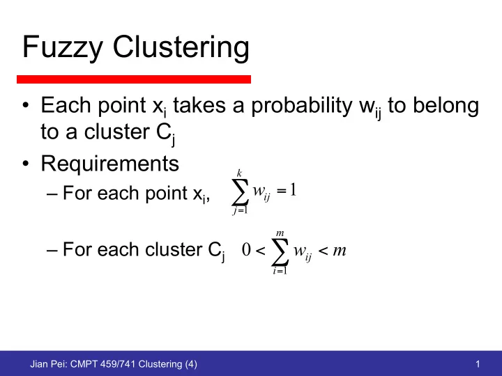
Fuzzy Clustering
- Each point xi takes a probability wij to belong
to a cluster Cj
- Requirements
– For each point xi, – For each cluster Cj
1
1
=
∑
= k j ij
w
m w
m i ij <
<∑
=1