From Real faces to Virtual faces Alberto Borghese Department of - PDF document

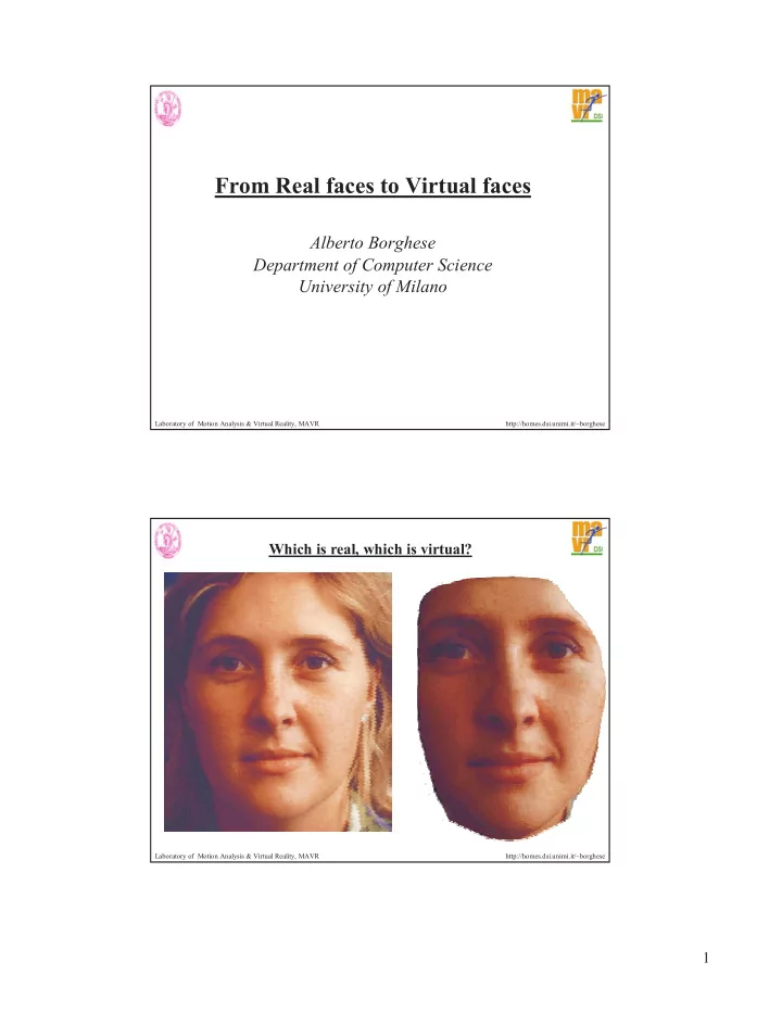
From Real faces to Virtual faces Alberto Borghese Department of Computer Science University of Milano Laboratory of Motion Analysis & Virtual Reality, MAVR http://homes.dsi.unimi.it/~borghese Which is real, which is virtual? Laboratory of Motion Analysis & Virtual Reality, MAVR http://homes.dsi.unimi.it/~borghese 1

General schema Points Acquisition Topological mesh Costruzione della Colored Mesh Topologica construction Topological Mesh Video Acquisition Color Fuzzy Application ANIMATION Connection Motion Capture Construction of a Control mesh Control Mesh Laboratory of Motion Analysis & Virtual Reality, MAVR http://homes.dsi.unimi.it/~borghese Outline •Points acquisition •From points to surface (mesh) •Mesh compression •Application of colour attribute •Animation Laboratory of Motion Analysis & Virtual Reality, MAVR http://homes.dsi.unimi.it/~borghese 2

Construction of the topological mesh Real object Digitization Sets of points Mesh construction (filtering) Sets of meshes Registration and fusion Single mesh Mesh compression (filtering) Final mesh Laboratory of Motion Analysis & Virtual Reality, MAVR http://homes.dsi.unimi.it/~borghese In-house Digitizers • Projection of patterns through a standard video projector. • Imaging through standard photocameras. • Image processing to extract range data points and texture. •There is some rigidity in the distribution of the range data. Laboratory of Motion Analysis & Virtual Reality, MAVR http://homes.dsi.unimi.it/~borghese 3

Minolta digitizers • Speed - scans in less than one second (Fast Mode) • Precision - over 300,000 points with range resolution to 0.0016" (Fine Mode) • Simplicity - point and shoot simplicity for consistently excellent results • Flexibility - only Minolta offers interchangeable lenses for variable scanning volumes http://www.minolta-3d.com/ Laboratory of Motion Analysis & Virtual Reality, MAVR http://homes.dsi.unimi.it/~borghese Face digitization (Autoscan) Acquisition session Points cloud Direct tessellation • Pair of video-cameras + standard laser pointer. • The range data are obtained by “painting” the surface manually. • Set of range data, which is denser where required. • High precision in spot localization (cross-correlation, bright image). Drawback: High scanning time. Direct tessellation produces an undesirable result. Laboratory of Motion Analysis & Virtual Reality, MAVR http://homes.dsi.unimi.it/~borghese 4

Digitization introduces errors Interpolation schemes (e.g. Delauney tessellation) fails because of measurement noise. ⇒ The need of filtering is evident. Laboratory of Motion Analysis & Virtual Reality, MAVR http://homes.dsi.unimi.it/~borghese How to convert the points into a mesh? Problem: noise Solution: regularized solutions. • Human body parts are “smooth” (lisce). • Noise has spatial frequencies higher that surface. • Surface has been over-sampled. Laboratory of Motion Analysis & Virtual Reality, MAVR http://homes.dsi.unimi.it/~borghese 5

HRBF Networks Incremental Reconstruction, error-driven. Laboratory of Motion Analysis & Virtual Reality, MAVR http://homes.dsi.unimi.it/~borghese Gaussian RBF Networks M ∑ z = s ( x ) = w k G ( x ; c k , Σ k ) Linear combination of Gaussian functions: k = 1 Pioneers in exploring properties of quasi-local units : •Broomhead e Lowe, 1988. •Moody e Darken, 1989. •Poggio e Girosi, 1990. •Park e Sandberg, 1991. Linear filtering : •Sanner and Slotine, 1992. •Canon and Slotine, 1995. •Borghese and Ferrari, 1996, 2001. •Poggio et al., 1993. •Canny, 1986 (Computer vision domain). Laboratory of Motion Analysis & Virtual Reality, MAVR http://homes.dsi.unimi.it/~borghese 6

Gaussian functions 2 − µ P P , µ ∈ R D 1 − ( ) µ σ = σ 2 G P ; | e π D / 2 σ D σ ∈ R Laboratory of Motion Analysis & Virtual Reality, MAVR http://homes.dsi.unimi.it/~borghese The RBF parameters M, µ k , σ k are the structural parameters. w j are the synaptic weights. Laboratory of Motion Analysis & Virtual Reality, MAVR http://homes.dsi.unimi.it/~borghese 7

Learning strategies • Empirical models: Broomhead and Lowe, 1988; Moody and Darken, 1989; Park and Sandberg, 1991. • Regularisation theory: Yuille e Grzywacz, 1988; Poggio and Girosi, 1990; Girosi et al., 1995; Wahba and Xu, 1998. The parameters: M, {P k } and σ k are set through an optimization process. Sparse approximation but non linear optimization- • Filtering Theory: Sanner e Slotine, 1992; Canon and Slotine 1995, Borghese and Ferrari, 1996, 2001; Canny, 1986. Laboratory of Motion Analysis & Virtual Reality, MAVR http://homes.dsi.unimi.it/~borghese Linear Gaussian filter M ∑ z = s ( x ) = w k G ( x ; c k , Σ k ) k = 1 − → Σ k= Σ ∀ k ( c c ) 0 Let us suppose: + k 1 k ∫ = − σ s ( x ) w ( c ) G (( x c ) | ) dc Continuos RBF: R STATEMENT 1: Let w(x), s(x) and G(x-c| σ ) ∈ L1(R) and be invariant to translation, then the continous RBF Network is equivalent to the convolution of the function w(x) with the Gaussian function: s(x) = w(x)*g(x; σ ) In the frequency domain: S( ν ) = W( ν ) G( ν;σ ) W(v) plays the role of a noisy version of S(v). Laboratory of Motion Analysis & Virtual Reality, MAVR http://homes.dsi.unimi.it/~borghese 8

Low-pass behavior of the Gaussian filter Pass band [0 ν cut-off ] Laboratory of Motion Analysis & Virtual Reality, MAVR http://homes.dsi.unimi.it/~borghese Discrete linear filter M ∑ z = s ( x ) = w k G ( x ; c k , Σ k ) c k+1 – c k = ∆ c ∀ c k Equally spaced Gaussians k = 1 Output: interpolation through the Gaussian basis Pass band [0 ν cut-off ] Stop band [ ν M ν s/2 ] v s = 1/ ∆ c Laboratory of Motion Analysis & Virtual Reality, MAVR http://homes.dsi.unimi.it/~borghese 9

Low-pass behavior of the Gaussian filter Pass band [0 ν cut-off ] Stop band [ ν M ν s/2 ] Laboratory of Motion Analysis & Virtual Reality, MAVR http://homes.dsi.unimi.it/~borghese Gaussian filtering Linear combination low-pass gaussian filter of gaussians single σ + M ∑ = ∗ − σ = σ s ( x ) w g ( x x ; ) s ( x ) w g ( x ; x , ) regular spacing k k k k k = k 1 M = ∑ l σ ∆ 2 S ( P ) z ( P ) G ( P ; P | ) P l kl kl l l = k 1 Laboratory of Motion Analysis & Virtual Reality, MAVR http://homes.dsi.unimi.it/~borghese 10

Linear filtering Artificial Vision. Filter grids which operate at different scales . Small scale (high frequency) Large scale (low frequency) ( ) ∑ M Linear combination of Basis Functions: = − σ S ( P ) S G P P | k k k Laboratory of Motion Analysis & Virtual Reality, MAVR 21 http://homes.dsi.unimi.it/~borghese HRBF Networks operation Quasi-local operations => Receptive field . •S(P k ) is estimated through a local weighted mean in the grid crossings: ∑ − σ S ( x ) G ( x x | ) m m m k = S ( P ) m ∑ k − σ G ( x x | ) m k m • x m belongs to the neighbourhood of G(x m -.|.) N ∑ = − σ s ( x ) S ( P ) G (( x x ); ) k k = k 1 Laboratory of Motion Analysis & Virtual Reality, MAVR http://homes.dsi.unimi.it/~borghese 11

Problem with this approach Single scale. 3D objects have different scales in different spatial locations. Small scale. There may be not enough points inside the receptive field of a Gaussian function. Small scale ⇒ Dense packing. Solutions: •Wavelets (from fine to coarse). •Adaptive hierarchical approach. Laboratory of Motion Analysis & Virtual Reality, MAVR http://homes.dsi.unimi.it/~borghese HRBF Networks Incremental s ( x ) Construction of the network a 1 ( x ) r 1 ( x ) a 2 ( x ) r 2 ( x ) r J ( x ) a J ( x ) noise ∑ r ( P ) 1 r ( ) ∈ P A P < ε r kl ≈ noise n N k Laboratory of Motion Analysis & Virtual Reality, MAVR http://homes.dsi.unimi.it/~borghese 12

HRBF Networks operation Quasi-local operations => Receptive field . •S(P k ) is estimated through a local weighted mean in the grid crossings: ∑ − σ S ( x ) G ( x x | ) m m m k = S ( P ) m ∑ k − σ G ( x x | ) m k m •A residual is computed for each measured point m as: R(P m ) = S(P m ) - S m (P m ) • The local reconstruction error is evaluated with a local integral metric ∑ for each crossing k as: − | R ( x ) S ( x ) | m m m MRE(P k ) = m N k Laboratory of Motion Analysis & Virtual Reality, MAVR http://homes.dsi.unimi.it/~borghese Hierarchical Radial Basis Function Network The surface is therefore reconstructed as: M L ∑∑ l = − σ S ( P ) w G (( P P ) | ) kl kl l = = l 1 k 1 Laboratory of Motion Analysis & Virtual Reality, MAVR http://homes.dsi.unimi.it/~borghese 13

Incremental Reconstruction Laboratory of Motion Analysis & Virtual Reality, MAVR http://homes.dsi.unimi.it/~borghese Sparse approximation Laboratory of Motion Analysis & Virtual Reality, MAVR http://homes.dsi.unimi.it/~borghese 14