
SLIDE 1
Frequentist Statistics and Hypothesis Testing
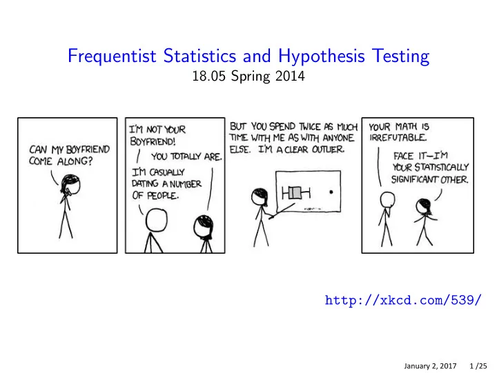
18.05 Spring 2014 http://xkcd.com/539/
January 2, 2017 1 /25
Frequentist Statistics and Hypothesis Testing 18.05 Spring 2014 - - PowerPoint PPT Presentation
Frequentist Statistics and Hypothesis Testing 18.05 Spring 2014 http://xkcd.com/539/ January 2, 2017 1 /25 Agenda Introduction to the frequentist way of life. What is a statistic? NHST ingredients; rejection regions Simple and composite
January 2, 2017 1 /25
January 2, 2017 2 /25
Yes: probability a coin lands heads. Yes: probability a given treatment cures a certain disease. Yes: probability distribution for the error of a measurement.
No: prior probability for the probability an unknown coin lands heads. No: prior probability on the efficacy of a treatment for a disease. No: prior probability distribution for the unknown mean of a normal
January 2, 2017 3 /25
January 2, 2017 4 /25
January 2, 2017 5 /25
January 2, 2017 6 /25
January 2, 2017 7 /25
January 2, 2017 8 /25
January 2, 2017 9 /25
January 2, 2017 10 /25
January 2, 2017 11 /25
January 2, 2017 12 /25
January 2, 2017 13 /25
January 2, 2017 14 /25
January 2, 2017 15 /25
January 2, 2017 16 /25
January 2, 2017 17 /25
January 2, 2017 18 /25
January 2, 2017 19 /25
January 2, 2017 20 /25
January 2, 2017 21 /25
January 2, 2017 22 /25
January 2, 2017 23 /25
January 2, 2017 24 /25
MIT OpenCourseWare https://ocw.mit.edu
Spring 2014 For information about citing these materials or our Terms of Use, visit: https://ocw.mit.edu/terms.