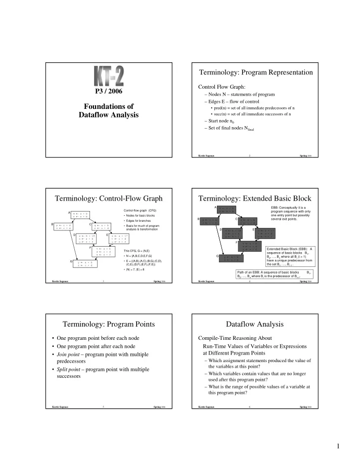
Foundations of pred(n) = set of all immediate predecessors of n - PDF document

Terminology: Program Representation Control Flow Graph: P3 / 2006 – Nodes N – statements of program – Edges E – flow of control Foundations of • pred(n) = set of all immediate predecessors of n Dataflow Analysis • succ(n) = set of all immediate successors of n – Start node n 0 – Set of final nodes N final Kostis Sagonas 2 Spring 2006 Terminology: Control-Flow Graph Terminology: Extended Basic Block A m � a + b EBB: Conceptually it is a Control-flow graph (CFG) n � a + b program sequence with only A m � a + b • Nodes for basic blocks one entry point but possibly n � a + b B C several exit points. p � c + d q � a + b • Edges for branches r � c + d r � c + d B C p � c + d q � a + b • Basis for much of program r � c + d r � c + d analysis & transformation D E e � b + 18 e � a + 17 s � a + b t � c + d D e � b + 18 E e � a + 17 u � e + f u � e + f s � a + b t � c + d u � e + f u � e + f F v � a + b w � c + d F v � a + b x � e + f Extended Basic Block (EBB): A w � c + d This CFG, G = (N,E) sequence of basic blocks B 1 , x � e + f • N = {A,B,C,D,E,F,G} G y � a + b B 2 , …, B n where all B i (i > 1) z � c + d have a unique predecessor from G • E = {(A,B),(A,C),(B,G),(C,D), y � a + b (C,E),(D,F),(E,F),(F,E)} the set B 1 , …, B i-1 . z � c + d • |N| = 7, |E| = 8 Path of an EBB: A sequence of basic blocks B 1 , B 2 , …, B n where B i is the predecessor of B i+1 . Kostis Sagonas 3 Spring 2006 Kostis Sagonas 4 Spring 2006 Terminology: Program Points Dataflow Analysis • One program point before each node Compile-Time Reasoning About • One program point after each node Run-Time Values of Variables or Expressions at Different Program Points • Join point – program point with multiple predecessors – Which assignment statements produced the value of the variables at this point? • Split point – program point with multiple – Which variables contain values that are no longer successors used after this program point? – What is the range of possible values of a variable at this program point? Kostis Sagonas 5 Spring 2006 Kostis Sagonas 6 Spring 2006 1

Dataflow Analysis: Basic Idea Forward Dataflow Analysis • Analysis propagates values forward through • Information about a program represented using control flow graph with flow of control values from an algebraic structure called lattice – Each node has a transfer function f • Analysis produces a lattice value for each • Input – value at program point before node program point • Output – new value at program point after node • Two flavors of analyses – Values flow from program points after predecessor nodes to program points before successor nodes – Forward dataflow analyses – At join points, values are combined using a merge – Backward dataflow analyses function • Canonical Example: Reaching Definitions Kostis Sagonas 7 Spring 2006 Kostis Sagonas 8 Spring 2006 Backward Dataflow Analysis Partial Orders • Analysis propagates values backward through • Set P • Partial order � such that � x,y,z � P control flow graph against flow of control – Each node has a transfer function f – x � x (reflexive) • Input – value at program point after node – x � y and y � x implies x � y (asymmetric) • Output – new value at program point before node – x � y and y � z implies x � z (transitive) – Values flow from program points before successor nodes to program points after predecessor nodes – At split points, values are combined using a merge function – Canonical Example : Live Variables Kostis Sagonas 9 Spring 2006 Kostis Sagonas 10 Spring 2006 Upper Bounds Lower Bounds • If S � P then • If S � P then – x � P is an upper bound of S if � y � S, y � x – x � P is a lower bound of S if � y � S, x � y – x � P is the least upper bound of S if – x � P is the greatest lower bound of S if • x is an upper bound of S, and • x is a lower bound of S, and • x � y for all upper bounds y of S • y � x for all lower bounds y of S – � - join , least upper bound (lub), supremum (sup) – � - meet , greatest lower bound (glb), infimum (inf) • � S is the least upper bound of S • � S is the greatest lower bound of S • x � y is the least upper bound of {x,y} • x � y is the greatest lower bound of {x,y} Kostis Sagonas 11 Spring 2006 Kostis Sagonas 12 Spring 2006 2

Coverings Example • Notation: x � y if x � y and x � y • P = {000, 001, 010, 011, 100, 101, 110, 111} (standard boolean lattice, also called hypercube) • x � y if (x bitwise_and y) = x • x is covered by y (y covers x) if We can visualize a partial – x � y, and 111 order with a Hasse Diagram – x � z � y implies x � z • If y covers x 011 110 101 • Line from y to x • Conceptually, y covers x if there are no 010 • y is above x in diagram elements between x and y 001 100 000 Kostis Sagonas 13 Spring 2006 Kostis Sagonas 14 Spring 2006 Lattices Top and Bottom • If x � y and x � y exist (i.e., are in P) for all x,y � P, • Greatest element of P (if it exists) is top ( T ) then P is a lattice . • Least element of P (if it exists) is bottom ( � ) • If � S and � S exist for all S � P, then P is a complete lattice . • Theorem: All finite lattices are complete • Example of a lattice that is not complete – Integers Z – For any x, y � Z, x � y = max(x,y), x � y = min(x,y) – But � Z and � Z do not exist – Z � { �� , �� } is a complete lattice Kostis Sagonas 15 Spring 2006 Kostis Sagonas 16 Spring 2006 Connection between � , � , and � Connecting Lemma Proofs (1) The following 3 properties are equivalent: • Proof of x � y implies x � y � y – x � y – x � y implies y is an upper bound of {x,y}. – x � y � y – Any upper bound z of {x,y} must satisfy y � z. – x � y � x – So y is least upper bound of {x,y} and x � y � y • Will prove: – x � y implies x � y � y and x � y � x • Proof of x � y implies x � y � x – x � y � y implies x � y – x � y implies x is a lower bound of {x,y}. – x � y � x implies x � y – Any lower bound z of {x,y} must satisfy z � x. • By Transitivity, – So x is greatest lower bound of {x,y} and x � y � x – x � y � y implies x � y � x – x � y � x implies x � y � y Kostis Sagonas 17 Spring 2006 Kostis Sagonas 18 Spring 2006 3

Connecting Lemma Proofs (2) Lattices as Algebraic Structures • Proof of x � y � y implies x � y • Have defined � and � in terms of � – y is an upper bound of {x,y} implies x � y • Will now define � in terms of � and � • Proof of x � y � x implies x � y – Start with � and � as arbitrary algebraic operations – x is a lower bound of {x,y} implies x � y that satisfy associative, commutative, idempotence, and absorption laws – Will define � using � and � – Will show that � is a partial order Kostis Sagonas 19 Spring 2006 Kostis Sagonas 20 Spring 2006 Connection Between � and � Algebraic Properties of Lattices Assume arbitrary operations � and � such that Theorem: x � y � y if and only if x � y � x – (x � y) � z � x � (y � z) (associativity of � ) • Proof of x � y � y implies x = x � y – (x � y) � z � x � (y � z) (associativity of � ) x = x � (x � y) (by absorption) – x � y � y � x (commutativity of � ) = x � y (by assumption) – x � y � y � x (commutativity of � ) • Proof of x � y � x implies y = x � y – x � x � x (idempotence of � ) y = y � (y � x) (by absorption) – x � x � x (idempotence of � ) = y � (x � y) (by commutativity) – x � (x � y) � x (absorption of � over � ) = y � x (by assumption) – x � (x � y) � x (absorption of � over � ) = x � y (by commutativity) Kostis Sagonas 21 Spring 2006 Kostis Sagonas 22 Spring 2006 Properties of � Properties of � • Define x � y if x � y � y • Proof of asymmetry property. Must show that x � y � y and y � x � x implies x � y • Proof of transitive property. Must show that x � y � y and y � z � z implies x � z � z x = y � x (by assumption) = x � y x � z = x � (y � z) (by assumption) (by commutativity) = (x � y) � z (by associativity) = y (by assumption) = y � z • Proof of reflexivity property. Must show that (by assumption) x � x � x = z (by assumption) x � x � x (by idempotence) Kostis Sagonas 23 Spring 2006 Kostis Sagonas 24 Spring 2006 4