{ Formally, we can characterize the 2D Moore neighbourhood c i ( t+ - - PDF document

formally we can characterize the 2d moore neighbourhood c
SMART_READER_LITE
LIVE PREVIEW

{ Formally, we can characterize the 2D Moore neighbourhood c i ( t+ - - PDF document

Two-Dimensional Cellular Automata 2 Christian Jacob, University of Calgary Two-dimensional CA Neighbourhoods Totalistic Cellular Automata Consider the following 1D CA rule: 111 110 101


slide-1
SLIDE 1

Christian Jacob, University of Calgary 2

Two-Dimensional Cellular Automata

Christian Jacob, University of Calgary 3

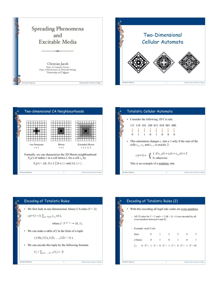
Formally, we can characterize the 2D Moore neighbourhood Nij(r) of radius r in a cell lattice L for a cell cij by

  • Nij(r) = {(k, l) L | |k-i| r and |l-j| r }.

Two-dimensional CA Neighbourhoods

von Neumann r = 1 Moore r = 1 Extended Moore r = 1, 2, 3

Christian Jacob, University of Calgary 4

Totalistic Cellular Automata

  • Consider the following 1D CA rule:

111 110 101 100 011 010 001 000 0 1 1 0 1 0 0 0

  • This automaton changes ci into a 1 only if the sum of the

cells ci-1, ci, and ci+1 is exactly 2: This is an example of a totalistic rule. ci(t+1) = 1, if ci-1(t) + ci(t) + ci+1(t) = 2 0, otherwise

{

Christian Jacob, University of Calgary 5

Encoding of Totalistic Rules

  • We first look at one-dimensional, binary CA rules (V = 2):

ci(t+1) = f ( j Ni(2) ci+j (t) ),

  • where f : V 2r +1 {0, 1}.
  • We can make a table of f in the form of a tuple
  • ( f (0), f (1), f (2), …, f (2r + 1) ).
  • We can encode this tuple by the following formula:
  • Cf = j=0, …, 2r+1 f ( j ) · 2j.

Christian Jacob, University of Calgary 6

Encoding of Totalistic Rules (2)

  • With this encoding all legal rule codes are even numbers.

– All 32 rules for V = 2 and r = 2 (K = 2r +1) are encoded by all even numbers between 0 and 62. – Example: mod-2 rule Sum: 1 2 3 4 5 f (Sum): 1 1 1 Cf : 0 · 20 + 1 · 21 + 0 · 22 + 1 · 23 + 0 · 24 + 1 · 25 = 42

slide-2
SLIDE 2

Christian Jacob, University of Calgary 7

Encoding of Totalistic Rules (3)

  • This encoding for binary, totalistic CAs (V = 2)
  • Cf = j=0, …, 2r+1 f ( j ) · 2j

can be generalized to any number of V values per cell:

  • Cf = j=0, …, 2r+1 f ( j ) · Vj ,

where f maps to any of the k values for a neighbourhood

  • f radius r:
  • f : {0, 1, …, 2r +1} {0, 1, …, V}.

Christian Jacob, University of Calgary 8

Some Example 2D Cellular Automata: 1022

5-neighbourhood, outer totalistic

0-39 40 30 20

Christian Jacob, University of Calgary 9

Some Example 2D Cellular Automata: 510

5-neighbourhood, outer totalistic

0-39 40 30 20

Christian Jacob, University of Calgary 10

Some Example 2D Cellular Automata: 374

5-neighbourhood, outer totalistic

0-39 40 30 20

Christian Jacob, University of Calgary 11

Some Example 2D Cellular Automata: 614

5-neighbourhood, outer totalistic

0-39 40 30 20

Christian Jacob, University of Calgary 12

Some Example 2D Cellular Automata: 174

5-neighbourhood, outer totalistic

0-39 40 30 20

slide-3
SLIDE 3

Christian Jacob, University of Calgary 13

Some Example 2D Cellular Automata: 494

5-neighbourhood, outer totalistic

0-39 40 30 20

Christian Jacob, University of Calgary 14

Patterns from Seed Regions: 143954

9-neighbourhood, outer totalistic

Single-Cell Seed Random Disordered Seed

Christian Jacob, University of Calgary 15

Patterns from Seed Regions: 50224

9-neighbourhood, outer totalistic

Single-Cell Seed Random Disordered Seed

Christian Jacob, University of Calgary 16

Patterns from Seed Regions: 15822

9-neighbourhood, outer totalistic

Single-Cell Seed Random Disordered Seed

Christian Jacob, University of Calgary 17

Patterns from Seed Regions: 85507

9-neighbourhood, outer totalistic

Single-Cell Seed Random Disordered Seed

Christian Jacob, University of Calgary 18

Patterns from Seed Regions: 191044

9-neighbourhood, outer totalistic

Single-Cell Seed Random Disordered Seed

slide-4
SLIDE 4

Christian Jacob, University of Calgary 19

Patterns from Seed Regions: 93737

9-neighbourhood, outer totalistic

Single-Cell Seed Random Disordered Seed

Christian Jacob, University of Calgary 20

Spreading Phenomena

Christian Jacob, University of Calgary 21

Spreading Phenomena

  • Spreading is the process in which an object extends itself
  • ver an increasingly larger area by incorporating regions

adjacent to itself.

  • The spreading or kinetic growth (KG) models describe a

wide variety of natural processes:

– Tumor growth – Epidemic spread – Gelation – Rumor-mongering – Fluid flow through porous media – …

Christian Jacob, University of Calgary 22

Slow Diffusive Growth: 256746

9-neighbourhood, outer totalistic

Christian Jacob, University of Calgary 23

Slow Diffusive Growth: 736

9-neighbourhood, outer totalistic

Christian Jacob, University of Calgary 24

Slow Diffusive Growth: 174826

9-neighbourhood, outer totalistic

slide-5
SLIDE 5

Christian Jacob, University of Calgary 25

Slow Diffusive Growth: 175850

9-neighbourhood, outer totalistic

Christian Jacob, University of Calgary 26

Eden Model

  • The original kinetic growth model was the Eden model,

introduced by the biologist M. Eden in the 1960s.

  • The Eden model simulates accretive growth of a cell

cluster (originally for simulating the spread of tumor cells) in a square lattice by sequentially adjoining randomly selected cells from the perimeter.

  • In more detail:

– We start with a cluster list consisting of a seed site. – A site is randomly chosen from the perimeter list, consisting of the nearest sites adjacent to the seed site (v. Neumann neighbourhood). – The cluster and perimeter lists are updated. – Another site is randomly selected from the perimeter list, and so on.

Christian Jacob, University of Calgary 27

Variations of the Eden Model

  • We look at two variations of the Eden model:

– The Invasion Percolation Model – The Single Percolation Cluster Model

Christian Jacob, University of Calgary 28

The Invasion Percolation Model

  • The invasion percolation model describes the flow of fluid

through porous media.

  • Invasion Percolation Algorithm:

– Each site in the perimeter list has a random number associated with it. – The cluster spreads by incorporating the perimeter site with the lowest associated random number.

  • This model describes a process of spreading that “follows

the path of least resistance.”

Christian Jacob, University of Calgary 29

Invasion Percolation Model: Spreading

Christian Jacob, University of Calgary 30

Invasion Percolation Model: Spreading (2)

slide-6
SLIDE 6

Christian Jacob, University of Calgary 31

The Single Percolation Cluster Model

  • The single (or random) percolation cluster model

describes the epidemic spread of disease.

  • Single Percolation Cluster Algorithm:

– Each randomly selected perimeter site has a probability p of joining the cluster. – If the selected site is placed in the cluster, it is removed from the perimeter list. – Even if the selected site is not placed in the cluster, it is removed from the perimeter list so that it cannot be chosen again later.

  • When p = 1, this model reduces to the Eden model.

Christian Jacob, University of Calgary 32

Single Percolation Cluster Model: p = 1.0

Christian Jacob, University of Calgary 33

Single Percolation Cluster Model: p = 1.0

Christian Jacob, University of Calgary 34

Single Percolation Cluster Model: p = 0.5

Christian Jacob, University of Calgary 35

Invasion vs. Single Percolation

Invasion Percolation Single Percolation

p = 1.0 p = 0.5

Christian Jacob, University of Calgary 36

Excitable Media

slide-7
SLIDE 7

Christian Jacob, University of Calgary 37

Excitable Media

  • Systems involving excitable media:

– Slime mold growth, – Star formation in spiral galaxies, – Cardiac tissue contraction, – Reaction-diffusion chemical systems, – Infectious disease epidemics

  • In each of these cases various spatially distributed patterns

are formed (such as concentric and spiral waves).

Christian Jacob, University of Calgary 38

Excitable Media (2)

  • Self-organized, self-propagating structures consist of

spatially distributed elements which

– can be excited as a result of interacting with neighbouring elements, – subsequently returning incrementally to the quiescent state in which they are again receptive to being excited.

  • The excited-refractory-receptive cycle characterizes these

systems.

  • These can be modeled using multi-state cellular automata.

Christian Jacob, University of Calgary 39

2D CA: Emergent Pattern Formation in Excitable Media

Neuron excitation Cyclic Space Hodgepodge

Christian Jacob, University of Calgary 40

Neuron Excitation

  • Electrical activity in biological systems can exhibit

excitable media behaviour.

  • Example: contraction of cardiac tissue (heart muscle)
  • The two-dimensional Greenberg-Hastings CA has been

used to model neuron excitation and recovery in a network

  • f neurons.

– Lattice site (neuron) values range from 1 to r. – A neuron with value 1 is said to be excited. – A neuron with value r is said to be rested. – A neuron with an intermediate value is said to be in a state of recovery.

Christian Jacob, University of Calgary 41

Neuron Excitation: Rules

  • In the neuron excitation-recovery process, an excited

neuron goes through a sequence of recovery states until it is rested.

  • A rested neuron becomes excited if at least one nearest

neighbour (v. Neumann) neuron is excited.

  • Update rules:

– A rested neuron (having value v = r) with at least one excited nearest neighbour neuron (having value v = 1) becomes excited (r 1). – A rested neuron (having value v = r) with no excited nearest neighbour remains rested (r r). – A neuron that is in a recovery state (1 v r-1) goes to the next recovery state (v v +1).

Christian Jacob, University of Calgary 42

Neuron Excitation: Rule Implementation

  • Here is an example of how to implement the Neuron

Excitation rules through pattern matching in Mathematica:

neuron[a_, b_, r, d_, e_]:= 1 /; MatchQ[1,a|b|d|e] neuron[a_, b_, r, d_, e_]:= r neuron[_, _, c_, _, _] := c + 1 Attributes[neuron]= Listable

slide-8
SLIDE 8

Christian Jacob, University of Calgary 43

Neuron Excitation: Visualization

Random Initial Configuration

Christian Jacob, University of Calgary 44

Neuron Excitation: Visualization

Christian Jacob, University of Calgary 45

Neuron Excitation: Visualization

Christian Jacob, University of Calgary 46

Cyclic Space

  • In the Greenberg-Hastings CA, the recovery of a site

proceeds independently of the state of neighbouring sites.

  • In the Cyclic Space CA, the recovery process for a site

proceeds only when a neighbouring site is slightly more relaxed.

  • The behaviour of this model has been related to the

changes that occur in phase transitions (e.g., water to ice).

Christian Jacob, University of Calgary 47

Cyclic Space: Rules

  • Lattice sites have values between 0 and n-1.
  • Update rules:

– A cell in state n-1 goes to state 0 if any of its nearest neighbour cells are in state 0. That is, a cell in state n-1 is “eaten” by a nearest neighbour cell in state 0. – A cell in state v, 0 v n-1, goes to state v +1 if any of its nearest neighbour cells is in state v +1. – A cell in state v, 0 v n -1, remains in state v if it has no nearest neighbour cell in state v +1.

Christian Jacob, University of Calgary 48

Cyclic Space: Rule Implementation

  • Here is an example of how to implement the Cyclic Space

rules through pattern matching in Mathematica:

cyclicSpace[a_, b_, (n-1), d_, e_]:= 0 /; MatchQ[0, a | b | d | e ] cyclicSpace[a_, b_, c_, d_, e_]:= (c+1) /; MatchQ[(c+1), a | b | d | e ] cyclicSpace[_, _, c_, _, _] := c Attributes[cyclicSpace]= Listable

slide-9
SLIDE 9

Christian Jacob, University of Calgary 49

Cyclic Space: Visualization

Random Initial Configuration

Christian Jacob, University of Calgary 50

Cyclic Space: Visualization

Christian Jacob, University of Calgary 51

Cyclic Space: Visualization

Christian Jacob, University of Calgary 52

Hodgepodge Machine

  • Hodgepodge = heterogeneous mixture
  • The Hodgepodge Machine models autocatalytic chemical

reactions.

  • Two or more compounds combine, dissociate, and

recombine in the presence of a catalyst.

  • Examples:

– Combination of carbon monoxide and oxygen to form carbon dioxide while these molecules are absorbed on the surface of dispersed palladium crystallites (catalytic converters in cars!). – Belousov-Zhabotinsky reaction: malonic acid is oxidized by potassium bromate in the presence of iron or cerium. – Spreading of infectious diseases.

Christian Jacob, University of Calgary

Belousov-Zhabotinsky Reaction

53

http://www.uni-regensburg.de/Fakultaeten/nat_Fak_IV/Organische_Chemie/Didaktik/Keusch/D-oscill-e.htm http://www.math.chalmers.se/~jacques/kf2na/Historia/Belousev.html

Christian Jacob, University of Calgary

The B-A-C Oscillating Reaction

The Blue/Amber/Colorless Oscillating Reaction

Demonstration: Three solutions are combined in alphabetical order.

  • Solution A: 30% H2O2 diluted in water.
  • Solution B: KIO3 dissolved in water, H2SO4

added, and diluted.

  • Solution C: Malonic acid and MnSO4 * H2O

dissolved in water, starch solution added, and diluted. Observations: The resulting solution turns from amber to blue-

  • black. The blue slowly fades to colorless, and the

reaction begins again. During the course of the reaction, bubbles are evolved.

54 http://chemed.chem.purdue.edu/demos/main_pages/22.8.html

slide-10
SLIDE 10

Christian Jacob, University of Calgary 55

Hodgepodge: Rules

  • s s square lattice with periodic boundary conditions.
  • Lattice site values range from 0 to r.
  • Cells having a value of 0 are said to be healthy.
  • Cells having a value r are said to be ill.
  • All other cells (0 < v < r) are said to be infected.

The higher the value, the more infected the cell is.

Christian Jacob, University of Calgary 56

Hodgepodge: Rules

  • Update rules:

– If a cell is ill (v = r), it becomes healthy (v 0). – If a cell is healthy (v = 0), it becomes infected with the new v determined by:

Min[r, Floor[# infected NN cells / k1 ] + Floor[# ill NN cells / k2 ]

  • where k1 and k2 are constants.

Note: The use of Min ensures that v does not exceed r. – If a cell is infected (0 < v < r), it becomes more infected with the new v determined by:

Min[r, g + Floor[sum of NN cell values / # infected NN cells ]

where g is an integer known as the speed of infection constant.

Christian Jacob, University of Calgary 57

Hodgepodge: Rule Implementation

  • Here is an example of how to implement the Hodgepodge

rules through pattern matching in Mathematica:

hodgepodge[r, _, _, _]:= 0 hodgepodge[0, x_, y_, _]:= Min[r, Floor[y/k1] + Floor[x/k2]] hodgepodge[c_, x_, y_, z_] := Min[r, g + Floor[(c+(r x) + z)/(y+1)]] Attributes[hodgepodge]= Listable

Christian Jacob, University of Calgary 58

Hodgepodge: Visualization

Random Initial Configuration

Christian Jacob, University of Calgary 59

Hodgepodge: Visualization

Christian Jacob, University of Calgary 60

Hodgepodge Machine: Visualization

slide-11
SLIDE 11

Christian Jacob, University of Calgary 61

References

  • Eden, M. (1960). A two-dimensional growth process . In Proceedings
  • f Fourth Berkeley Symposium on Mathematics, Statistics, and

Probability, volume 4, pages 223-239, Berkeley, 1960. University of California Press.

  • Gaylord, R. J. and P. R. Wellin (1995). Computer Simulations with

MATHEMATICA: Explorations in Complex Physical and Biological Systems. New York, Springer. (in particular: chapters 4 and 11).

  • Gaylord, R. J. and K. Nishidate (1996). Modeling Nature: Cellular

Automata Simulations with Mathematica. New York, TELOS/Springer.

  • Toffoli, T. and N. Margolus (1987). Cellular Automata Machines: A New

Environment for Modeling, MIT Press.

  • Wolfram, S. (1994). Cellular Automata and Complexity. Reading,

Addison-Wesley.

  • Wolfram, S. (2002). A New Kind of Science. Champaign, IL, Wolfram

Media.