For our snacks price index problem, this is 10 * 15 + 10 * 15 300 - PowerPoint PPT Presentation

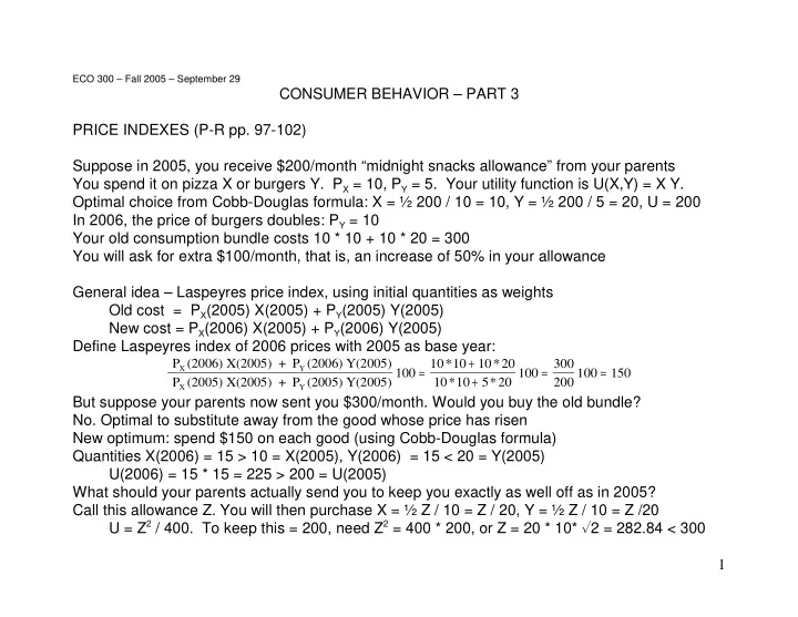
ECO 300 – Fall 2005 – September 29 CONSUMER BEHAVIOR – PART 3 PRICE INDEXES (P-R pp. 97-102) Suppose in 2005, you receive $200/month “midnight snacks allowance” from your parents You spend it on pizza X or burgers Y. P X = 10, P Y = 5. Your utility function is U(X,Y) = X Y. Optimal choice from Cobb-Douglas formula: X = ½ 200 / 10 = 10, Y = ½ 200 / 5 = 20, U = 200 In 2006, the price of burgers doubles: P Y = 10 Your old consumption bundle costs 10 * 10 + 10 * 20 = 300 You will ask for extra $100/month, that is, an increase of 50% in your allowance General idea – Laspeyres price index, using initial quantities as weights Old cost = P X (2005) X(2005) + P Y (2005) Y(2005) New cost = P X (2006) X(2005) + P Y (2006) Y(2005) Define Laspeyres index of 2006 prices with 2005 as base year: P (2006) X(2005) + P (2006) Y(2005) + 10 10 * 10 20 * 300 X Y = = = 100 5 20 100 200 100 150 + P (2005) X(2005) + P (2005) Y(2005) 10 10 * * X Y But suppose your parents now sent you $300/month. Would you buy the old bundle? No. Optimal to substitute away from the good whose price has risen New optimum: spend $150 on each good (using Cobb-Douglas formula) Quantities X(2006) = 15 > 10 = X(2005), Y(2006) = 15 < 20 = Y(2005) U(2006) = 15 * 15 = 225 > 200 = U(2005) What should your parents actually send you to keep you exactly as well off as in 2005? U = Z 2 / 400. To keep this = 200, need Z 2 = 400 * 200, or Z = 20 * 10* % 2 = 282.84 < 300 Call this allowance Z. You will then purchase X = ½ Z / 10 = Z / 20, Y = ½ Z / 10 = Z /20 1

True index = (282.84/200)*100 = 141.42 < 150; Laspeyres index overstates the price increase This is one reason for the “upward bias in the CPI” recently much discussed in policy debates (Other reasons – quality improvements, cheap outlets not properly accounted for) An alternative, the Paasche index, uses the current or final year quantities as weights: P (2006) X(2006) + P (2006) Y(2006) X Y 100 P (2005) X(2006) + P (2005) Y(2006) X Y For our snacks price index problem, this is 10 * 15 + 10 * 15 300 = = < 10* 15 + 5 * 15 100 225 100 13333 . 14142 . So the Paasche index understates the true change in the cost of living If all prices increased in the same proportion (“pure inflation”), e.g if in 2006, P X = 20, P Y = 10 P (2006) X(2005) + P (2006) Y(2005) + 20 10 * 10 10 * Laspeyres index is X Y = = 100 5 10 100 200 + P (2005) X(2005) + P (2005) Y(2005) 10 10 * * X Y And calculation of the income Z needed to maintain 2005 utility is X = ½ Z / 20 = Z / 40, Y = ½ Z / 10 = Z / 20, U = Z 2 / 800 To keep this = 200, need Z 2 = 800 * 200 = 400 * 400, or Z = 400 so no bias. Similarly Paasche index has no bias in this situation either So “pure inflation” is the easy case; changes in RELATIVE prices cause biases in price indexes Precisely because substitution occurs in response to changes in relative prices That is why “CPI bias” problem was so big in recent years – big relative price changes One solution – chaining. Each year, use last year’s quantities as weights Relative price changes over one year are small, so errors small 2

MARKET DEMAND (P-R pp. 122-7, 132-4) Horizontal sum of individual demands. Example: Two consumers A and B Individual demands Q A = a - c P, Q B = b - d P Market demand Q = Q A + Q B = (a+b) - (c+d) P when P < a/c This works so long as these are independent But may have interactive effects – positive or negative Consider example of positive – fashion or networks Q A = 12 - 2 P + 0.5 Q B , Q B = 12 - 2 P + 0.5 Q A Solve these jointly: Q A = 24 - 4 P , Q B = 24 - 4 P , Total Q = Q A + Q B = 48 - 8 P Additional effect of prices because lower price has a direct effect on quantities, then a further effect of each quantity on the other, then a third round, ... Total effect is the cumulation of all these Definitions and calculations of price elasticities of market demand same as for individual ones Formally, can also calculate elasticity of market demand with respect to total income But doing and interpreting this needs some care: Redistribution of income may alter individual demands unequally, and therefore change total demand For necessities, more equal income distribution causes increase in quantity demanded, for luxuries, a decrease 3

PRICE ELASTICITIES THROUGH TIME (P-R pp. 38-43) Usual presumption – price elasticities of demand higher in the long run than in the short Intuition – with more time, the consumers [1] are better informed about the price change, [2] learn better how to cope with new goods, change habits, [3] are less bound by previous commitments or contracts, ... Therefore we should see larger quantity response the longer the run This is broadly correct. But need more thought, and more precise specification [1] Is the price change temporary or permanent? [2] Is the good in question non-durable or durable? If non-durable, how substitutable over time? For durables, short-run elasticity often > long-run elasticity following permanent price change Example: 1000 people, each buys 1 car, keeps for 5 years. In the original “steady state” of the system, annual quantity demanded = 200 Now price drops. Each buys 1.2 cars (on average), keeps for 4 years In the new “steady state”, annual quantity demanded = 300 But in the first year, two cohorts (200 owners of 5-year-olds, 200 of 4-year-olds) replace their cars, plus the 200 who are going to buy a second car do so. Quantity = 600 In the second, third, and fourth years, back down to 200. Fifth year, back up to 600. So new steady state may not even be reached; instead “echo” of initial impact. In practice, the echo is gradually flattened by various uncertainties; go to new steady state. For temporary price changes, large effect if good is durable or substitutable over time Examples – sales, “happy hours” or “early-bird specials” 4

EMPIRICAL ESTIMATION – ISSUES (P-R 136-40) [1] Choice of level of aggregation – over consumers, and over commodities Often dictated by data availability and computational complexities Increasingly, large samples of individual households’ choices available Commodity data still quite coarsely aggregated except for specific marketing studies Computer power increasing rapidly [2] Functional form specification – linear, logarithmic ... ? Each imposes implicit assumptions about substitution etc. Richer the form, the more we can estimate parameters from data rather than impose But too many parameters leave too few degrees of freedom. [3] Scope of estimation – do you include saving, labor supply etc. [4] Biggest problem – estimates are biased if there are feedbacks from quantities to the supposed explanatory (exogenous) variables. Example: Two data points, R and G Prices P R , P G differ because higher tax in G Why is the tax higher in G? Could be because demand is higher G than in R (D G upward shift of D R ) Economist might see points G, R and fit D E But that would be wrong: too inelastic Lesson — understand your data and reasons for variation you see Look for “experiments” in data: “control group” and “treatment group” that differ only in the aspect you want to focus on 5

EMPIRICAL ESTIMATION – EXAMPLE From Richard Blundell, “Consumer Behavior: Theory and Empirical Evidence,” Economic Journal, March 1988 Recognizes n = 6 commodity classifications. Prices P k , quantities Q k , income I Dependent variables – expenditure shares S k = ( P k Q k ) / I Data – expenditure survey of 65,000 U.K. households (those sampled are required to keep detailed notebooks on their spending) ⎡ ⎤ α / 2 ⎛ ⎞ α ⎛ ⎞ / 2 P P P Q P P n n n ∑ θ ∑ ∑ ⎜ ⎟ ⎢ ⎥ ⎜ ⎟ i j = = + β − θ k k i k S 1 ⎝ ⎠ ⎝ ⎠ k ik k ij 2 ⎢ 2 ⎥ I I I ⎣ ⎦ = = = i 1 i 1 j 1 No need to remember this, but note that applied economics needs a lot of math By fitting these formulas to the data, he estimates the “parameters” " , $ k , 2 ij Results shown in tables on last two pages of handout Note – in the tables, “compensated” means considering only the pure substitution effect, with income adjusted to keep the consumer on the original indifference curve “uncompensated” means the total effect, holding money income constant Results give considerably detailed information about income elasticities (budget elasticities) and price elasticities – “compensated” ones correspond to pure substitution effects, “uncompensated” ones correspond to total effects of the price changes 6