[PPT] - Folk theorems, myths, & conjectures Christiaan Huygens (1629 PowerPoint Presentation

SLIDE 1

Folk theorems, myths, & conjectures in complex oscillator networks

NetSci 2015 Satellite Symposium

Florian D¨

rfler

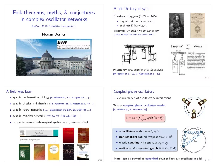
A brief history of sync

Christiaan Huygens (1629 – 1695) physicist & mathematician engineer & horologist

bserved “an odd kind of sympathy ”

[Letter to Royal Society of London, 1665]

Recent reviews, experiments, & analysis

[M. Bennet et al. ’02, M. Kapitaniak et al. ’12]

2 / 27

A field was born

sync in mathematical biology [A. Winfree ’80, S.H. Strogatz ’03, . . . ] sync in physics and chemistry [Y. Kuramoto ’83, M. M´

ezard et al. ’87. . . ]

sync in neural networks [F.C. Hoppensteadt and E.M. Izhikevich ’00, . . . ] sync in complex networks [C.W. Wu ’07, S. Bocaletti ’08, . . . ] . . . and numerous technological applications (reviewed later)

Physics Reports 469 (2008) 93–153 Contents lists available at ScienceDirect

Physics Reports

journal homepage: www.elsevier.com/locate/physrep

Synchronization in complex networks

Alex Arenas a,b, Albert Díaz-Guilera c,b, Jurgen Kurths d,e, Yamir Moreno b,f,∗, Changsong Zhou g

a

3 / 27

Coupled phase oscillators

∃ various models of oscillators & interactions Today: coupled phase oscillator model

[A. Winfree ’67, Y. Kuramoto ’75]

˙ θi = ωi − n

j=1 aij sin(θi −θj) ◮ n oscillators with phase θi ∈ S1 ◮ non-identical natural frequencies ωi ∈ R1 ◮ elastic coupling with strength aij = aji ◮ undirected & connected graph G = (V, E, A)

ω1 ω3 ω2 a12 a13 a23

Note: can be derived as canonical coupled limit-cycle oscillator model

4 / 27

SLIDE 2

My application of interest: sync in AC power networks

sync is crucial for AC power grids – a coupled oscillator analogy sync is a trade-off weak coupling & heterogeneous strong coupling & homogeneous

5 / 27

My application of interest: sync in AC power networks

sync is crucial for AC power grids – a coupled oscillator analogy sync is a trade-off weak coupling & heterogeneous Blackout India July 30/31 2012

5 / 27

Other technological applications of phase oscillators

particle filtering to estimate limit cycles [A. Tilton & P. Mehta et al. ’12] clock synchronization over networks

[Y. Hong & A. Scaglione ’05, O. Simeone et

al. ’08, Y. Wang & F. Doyle et al. ’12]

central pattern generators and robotic locomotion [J. Nakanishi et al.

’04, S. Aoi et al. ’05, L. Righetti et al. ’06]

decentralized maximum likelihood estimation [S. Barbarossa et al. ’07] carrier sync without phase-locked loops [M. Rahman et al. ’11] robotic vehicle coordination

[R. Sepulchre et al. ’07, D. Klein et al. ’09]

s1(t) VCO PD (s) ε 1 T1 ∆Φ1(t) s2(t) (s) ε VCO 1 T2 ∆Φ2(t) PD VCO s3(t) ∆Φ3(t) PD 1 T3 (s) ε

(x, y) θ

θ

6 / 27

Phenomenology and challenges in synchronization

many fundamental questions are still open

Transition to synchronization is a trade-off: coupling vs. heterogeneity Some central questions: (still after 45 years of work) quantify “coupling” vs. “heterogeneity” multiple sync’d states & their sync basin interplay of network & dynamics In more technical terms: existence, uniqueness, & stability of equilibria and their basin of attraction . . . as a function of network topology & parameters

7 / 27

SLIDE 3

Outline

Introduction Synchronization Threshold Equilibrium Landscape Almost Global Synchronization Conclusions I try to shed light on some fundamental yet poorly understood questions.

Main references today

Automatica 50 (2014) 1539–1564

Contents lists available at ScienceDirect

Automatica

journal homepage: www.elsevier.com/locate/automatica

Survey paper

Synchronization in complex networks of phase oscillators: A survey

I

Florian Dörfler a,1, Francesco Bullo b

a Automatic Control Laboratory, ETH Zürich, Switzerland b Department of Mechanical Engineering, University of California Santa Barbara, USA

Algebraic geometrization of the Kuramoto model: Equilibria and stability analysis

Dhagash Mehta,1,a) Noah S. Daleo,2,b) Florian D€

rfler,3,c) and Jonathan D. Hauenstein1,d)

1Department of Applied and Computational Mathematics and Statistics, University of Notre Dame, Notre

Dame, Indiana 46556, USA

2Department of Mathematics, North Carolina State University, Raleigh, North Carolina 27695, USA 3Automatic Control Laboratory, Swiss Federal Institute of Technology (ETH) Z€

urich, 8092 Z€ urich, Switzerland CHAOS 25, 053103 (2015)

8 / 27

Models & sync notion

finite dimensional & heterogeneous

uniform all-to-all Kuramoto model ˙ θi = ωi − n

j=1

K n sin(θi − θj) where K > 0 is the coupling strength among the oscillators general coupled oscillator model ˙ θi = ωi − n

j=1 aij sin(θi − θj)

where aij = aji ≥ 0 induces a connected and undirected graph Frequency synchronization: ˙ θi = ωsync ∈ R for all i ∈ {1, . . . , n} Lemma: if there is a frequency-sync’d solution, then ωsync = n

i=1 ωi/n

⇒ frequency-synchronized solutions are equilibria in rotating coordinates

9 / 27

the synchronization threshold

r existence, uniqueness, &

local stability of equilibria

SLIDE 4

Synchronization threshold for the complete graph

˙ θi = ωi − n

j=1

K n sin(θi − θj) synchronization if K > Kcrit(ω) ⇒ necessary & tight lower bound [Chopra & Spong ’09] Kcrit ≥ max

i,j 1 2 |ωi − ωj|

⇒ sufficient & tight upper bound [FD & Bullo ’11] Kcrit ≤ max

i,j |ωi − ωj|

ωmax ωmin p (1 − p) ω π/2 1 n 1 n ω −ω0 +ω0 n − 2 n π/2 π/2 gtrip,n(ω) gbip(ω)

tight lower bound tight upper bound

10 / 27

Synchronization threshold for the complete graph – cont’d

1 explicit & tight lower/upper bounds [Chopra & Spong ’09, FD & Bullo ’11]

1 2 maxi,j |ωi − ωj| ≤ Kcrit ≤ maxi,j |ωi − ωj|

2 exact & implicit [Aeyels & Rogge ’04, Mirollo & Strogatz ’05, Verwoerd & Mason ’08]

Kcrit =

nu∗ n

i=1

√

1−(ωi/u∗)2 where u∗ ∈ [ω∞ , 2 ω∞] is the unique

solution to the equation 2 n

i=1

1 − (ωi/u)2 = n

i=11/

1 − (ωi/u)2 .

comparison of bounds for uniform distribution gunif (ω) ∈ [−1, +1]

n 4/π Kcrit

10

1

10

2

0.6 0.8 1 1.2 1.4 1.6 1.8 2

exact & implicit lower explicit upper explicit Kuramoto’s continuum limit bound

11 / 27

there’s nothing more to say for the complete uniform graph . . . so let’s move on

Primer on algebraic graph theory

Laplacian matrix L = “degree matrix” − “adjacency matrix” L = LT =     

. . . ... . . . ... . . . −ai1 · · · n

j=1 aij

· · · −ain . . . ... . . . ... . . .

     ≥ 0 Notions of connectivity spectral: 2nd smallest eigenvalue of L is “algebraic connectivity” λ2(L) topological: degree n

j=1 aij or degree distribution

Notions of heterogeneity ωE,∞ = max{i,j}∈E |ωi − ωj|, ωE,2 =

{i,j}∈E |ωi − ωj|21/2

12 / 27

SLIDE 5

Synchronization threshold in sparse networks

a brief overview on theoretical guarantees

˙ θi = ωi − n

j=1 aij sin(θi − θj)

1 necessary sync condition:

n

j=1 aij ≥ |ωi|

⇐ sync

[C. Tavora and O.J.M. Smith ’72]

2 sufficient sync condition:

λ2(L) > ωE,2 ⇒ sync

[FD and F. Bullo ’12]

⇒ ∃ similar conditions with diff. metrics on coupling & heterogeneity ⇒ Problem: sharpest general conditions are conservative

13 / 27

Nearly exact synchronization threshold

[FD, Chertkov, & Bullo ’12]

L†ω
E,∞ < 1

= ⇒ locally exponentially stable synchronization for 1) extremal topologies: acyclic, complete graphs, or {3, 4} rings 2) extremal parameters: L†ω is bipolar, small, or symmetric (for rings) 3) arbitrary one-connected combinations of 1) and 2) 4) with high probability, accuracy, & confidence “for almost all” G & ω intuition: cond’

L†ω
E,∞ < 1 includes previous λ2, degree, & complete:
eigenvectors of L


    . . . . . . 1/λ2(L) . . . . . . ... ... ... . . . . . . 1/λn(L)     

eigenvectors of L

T ω

E,∞

< 1

14 / 27

Nearly exact synchronization threshold – cont’d

Comparison with numerical Kcrit for ˙ θi = ωi −K ·n

j=1 aij sin(θi −θj)

0.1 0.4 0.7 1 0.75 0.9 1

Knumeric/Kanalytic

0.25 0.5 0.75 1 0.75 0.9 1

p K

0.25 0.5 0.75 1 0.75 0.9 1

p K

0.1 0.4 0.7 1 0.75 0.9 1

p

0.25 0.5 0.75 1 0.75 0.9 1

p K

Knumeric/Kanalytic

p

0.25 0.5 0.75 1 0.75 0.9 1

p K

Knumeric/Kanalytic

p

Knumeric/Kanalytic Knumeric/Kanalytic

p

Knumeric/Kanalytic

n = 10 n = 20 n = 40 n = 80 n = 160 p

ω uniform ω bipolar Small World Network Erd¨

s-R´

enyi Graph Random Geometric Graph

p

⇒ condition

L†ω
E,∞ < 1 is highly accurate & always guarantees sync

15 / 27

The synchronization threshold

Conjecture 1:

L†ω
E,∞ < 1 ⇒ exists locally exponentially stable sync

Monte Carlo:

L†ω
E,∞ < 1 =

⇒ sync “for almost all” G & ω

thin 0.03% set of counter-examples with O(10−4) error analytic counter-example with a large ring [FD, Chertkov, & Bullo ’12]

Many related problems are actually NP-hard: throughput maximization in capacitated network flow [A. Verma, ’09] power dispatch optimization [K. Lehmann, A. Grastien, & P. Van Hentenryck, ’14] finding non-zero stable equilibria of the Kuramoto model [R. Taylor, ’15] finding stable equilibria of the repulsive Kuramoto model [A. Sarlette, ’11] The conjecture is rejected. The sync threshold remains open & hard(?). . .

16 / 27

SLIDE 6

The problem may be hopeless . . . but the bounds ain’t bad

˙ θi = ωi − K · n

j=1 aij sin(θi − θj)

necessary & “sufficient” sync bounds: maxi n

j=1 aij

|ωi| ≤ Kcrit ≤

L†ω
E,∞

(exact for acyclic and tight for complete) ⇒ comparison w/ coarse numerical Kcrit

cycles (in tens of thousands)

1 2 3 4 5 6 7 8 9 10

c

0.5 1 1.5 2 2.5 3 3.5 4 4.5 5 5.5 6

Avg. theoretic UB
Avg. upper bound
Avg. lower bound
Avg. theoretic LB

Kcrit # cycles (in 104)

!"#$%&'()*%+',-. !"#$%/0)'*)/12%34

Avg. num. bound (up)
Avg. theo. bound (up)
Avg. num. bound (up)
Avg. theo. bound (low)

working horse: algebraic geometry [D. Mehta, N. Daleo, FD, & J. Hauenstein, ’15] ωi = n

j=1 aij sin(θi − θj) si=sin(θi)

⇐ = = = = ⇒

ci=cos(θi)

ωi = n

j=1 aij (sicj − sjci)

17 / 27

more fun with stable equilibria

Systems without stable equilibria

Conjecture 2: if there are any equilibria, then at least one must be stable equilibria of a ring graph with n = 10 & ωi ∈ [−1, 1] uniformly ˙ θi = ωi − K sin(θi − θi−1) − K sin(θi − θi+1) ⇒ multi-stable cases ⇒ all unstable for K = 13 − 15 ⇒ analytic counterexample by

[A. Araposthatis et al., ’81]

The conjecture is rejected.

50 100 200 400 600 800 1000 1200 number of equilibria K 50 100 0.5 1 1.5 2 2.5 3 number of stable equilibria K 1 2 3 4 5 6 7 8 9 10 1 2 3 4 5 6 7 8 9 10 1 2 3 4 5 6 7 8 9 10

18 / 27

How many stable equilibria are there?

acyclic graphs have a single stable equilibrium [FD, Chertkov, & Bullo ’12] previously: rings have multi-stable equilibrium landscapes complete graphs have a single stable equilibrium [Aeyels & Rogge ’04] Conjecture 3: the plot of # stable equilibria vs. cycles is a concave curve

# stable equilibria # cycles ring tree complete

number of cycles

10 20

average number of stable equilibria

1 1.02 1.04 1.06 1.08 1.1 1.12 1.14 1.16 1.18 1.2

variance

The conjecture is rejected & the problem is more puzzling.

19 / 27

SLIDE 7

A popular folk theorem about the “π/2-box”

Stable π/2-box: any equilibrium in

θ ∈ Tn : |θi − θj| < π/2 ∀{i, j} ∈ E
is locally exponentially stable (modulo rotational symmetry).

Proof: linearization is ˙ θ = −L(θ∗) · θ where L(θ∗) is a Laplacian:

L(θ∗) =       . . . ... . . . ... . . . −ai1 cos(θ∗

i − θ∗ 1)

· · · n

j=1 aij cos(θ∗ i − θ∗ j )

· · · −ain cos(θ∗

i − θ∗ n)

. . . ... . . . ... . . .      

⇒ a major part of the literature focuses on the π/2-box

Conjecture 4: there is at most one equilibrium in the π/2-box has been proved . . . at least on Rn [A. Araposthatis et al., ’81, K. Dvijotham et al., ’15]

20 / 27

The “π/2-box” does not guarantee uniqueness on Tn

Stable π/2-box: any equilibrium in

θ ∈ Tn : |θi − θj| < π/2 ∀{i, j} ∈ E
is locally exponentially stable (modulo rotational symmetry).

Conjecture 4: there is at most one equilibrium in the π/2-box Homogeneous counterexample ˙ θi = − sin(θi − θi−1) − sin(θi − θi+1) admits two equilibria in π/2-box (does not work in Rn) The conjecture is rejected on Tn.

27 27 27 27 27

θ5 = 0 θ5 = 4π 5 θ4 = 0 θ4 = 3π 5 θ2 = 0 θ2 = π 5 θ3 = 0 θ3 = 2π 5 θ1 = 0 1 2 3 4 5

21 / 27

Equilibrium indices in the Kuramoto model

Equilibria of the Kuramoto model & their indices (# stable eigenvalues) ˙ θi = ωi − n

j=1

K n sin(θi −θj)

10 10

1

10

2

10 10

1

10

2

10

3

10

4

10

5

K number of equilibria N=18 N=17 N=16 N=15 N=14 N=13 N=12 N=11 N=10 N=9 N=8 N=7 N=6 N=5 N=4 N=3

converge to 2n as K → ∞

5 10 15 10 10

1

10

2

10

3

10

4

10

5

index number of equilibria N=18 N=17 N=16 N=15 N=14 N=13 N=12 N=11 N=10 N=9 N=8 N=7 N=6 N=5 N=4 N=3

for K = 100 Conjecture 5 (open): for n & K large, there are n

j

equilibria of index j

22 / 27

(almost) global stability = sync basin is almost all of Tn

SLIDE 8

Conjecture for acyclic & undirected networks

Conjecture 6 for acyclic networks: if there is a locally exponentially stable equilibrium, then it is almost globally stable. Partial proof: conjecture is true for homogeneous ωi [P. Monzon, ’06] & can be extended to weakly heterogeneous cases via ISS [Angeli & Praly,’11]. Numerics: randomized simulations apparently always confirm conjecture.

23 / 27

Non-rigorous reasoning for acyclic networks

Transformation to branch coordinates ˙ θi = ωi − n

j=1 aij sin(θi − θj) δij=θi−θj

⇐ = = = = ⇒

∀{i,j}∈E

    . . . ˙ δij . . .     = Q     . . . ˜ ωij − sin(δij) . . .     , where Q is a positive definite matrix distorting the decoupled vector field.

y y´ = 0.3-sin(y)

3
2.5
2
1.5
1
0.5

0.5 1 1.5 2 2.5 3

3
2.5
2
1.5
1
0.5

0.5 1 1.5 2 2.5 3 y y´ = 2*(0.3-sin(y)) - 0.1*(0.5-sin(x))

3
2.5
2
1.5
1
0.5

0.5 1 1.5 2 2.5 3

3
2.5
2
1.5
1
0.5

0.5 1 1.5 2 2.5 3

24 / 27

Conjecture for acyclic networks is partially rejected

Conjecture 6 for acyclic networks: if there is a locally exponentially stable equilibrium, then it is almost globally stable. a 3-node counterexample by

[A. Gushchin, E. Mallada, & A. Tang, ’15]:

˙ θi = ωi − 3 · 3

j=1 aij sin(θi − θj)

27 27 27

1 2 3

ω1 = 2 − ε ω2 = ω3 = −1 + ε/2

δ13 δ12 −π +π +π reveals continua of limit cycles The conjecture is rejected, and the problem is now even more interesting due to partial proof for weakly heterogeneous oscillators. Possibly generic?

25 / 27

Complete & uniform (Kuramoto) networks

Conjecture 7 for complete networks: if there is a locally exponentially stable equilibrium, then it is almost globally stable. ˙ θi = ωi − K n · n

j=1 sin(θi − θj)

Today the conjecture is still open. Partial proofs: conjecture is true for homogeneous ωi [P. Monzon, ’06] & can be extended to weakly heterogeneous cases via ISS [Angeli & Praly,’11]. The semi-circle is know to be a subset of the sync basin [FD & F. Bullo, ’11]. Numerics: randomized simulations apparently always confirm conjecture. Plausible argument based on order parameter reiψ = n

j=1 1 neiθj

˙ θi = ωi − n

j=1 aij sin(θi − θj)

⇐ ⇒ ˙ θi = ωi − Kr sin(θi − ψ) This should essentially behave like a single oscillator system . . .

26 / 27

SLIDE 9

conclusions

Summary and conclusions

We rejected some conjectures systems without stable equilibria non-unique equilibria in π/2-box non-trivial sync basin for trees synchronization threshold bounds Acknowledgements: Dhagash Mehta, Noah Daleo, Jonathan Hauenstein, Francesco Bullo, John Simpson-Porco, Michael Chertkov, Matthias Rungger, Julien Hendrickx, Rodolphe Sepulchre, Fulvio Forni, . . . & found some intriguing problems: # stable equilibria vs. # cycles scaling of equilibrium indices almost global sync basin exact synchronization threshold “Surprisingly enough, this seemingly

bvious

fact seems difficult to prove.”

[Y. Kuramoto, ’84]

27 / 27