[PPT] - Finite Mathematics MAT 141: Chapter 1 Notes Slopes and Equations of PowerPoint Presentation

SLIDE 1

1/18/2012 1

Finite Mathematics MAT 141: Chapter 1 Notes

David J. Gisch January 10, 2012

Slopes and Equations of Lines.

Recall the Cartesian Plane

René Descartes 1596-1650

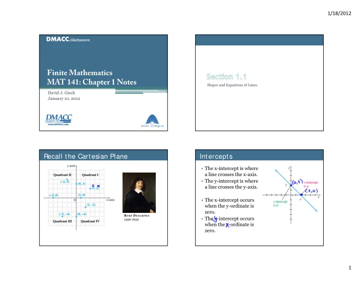
Intercepts

The x-intercept is where

a line crosses the x-axis.

The y-intercept is where

a line crosses the y-axis.

The x-intercept occurs

when the y-ordinate is zero.

The x-intercept occurs

when the y-ordinate is zero.

SLIDE 2

1/18/2012 2

S lope

The order of the subscripts does not matter as

long as you are consistent.

S lope

Example 1.1.1 Find the slope of the line.

S lope

Example 1.1.2: What is the slope of the line with the following properties?

(a) passes through 2, 3 and 4, 1 (b) passes through 3, 5 and has an x-intercept of 5.

S lope

SLIDE 3

1/18/2012 3

Equations of Lines S pecial Cases S ummary of Equations Equation of a Line

Example 1.1.3 Find the slope of the line. (a) 2 10 (b) 4 8 24 (c) Horizontal and through 2.2, 5.875

SLIDE 4

1/18/2012 4

Equation of a Line

Example 1.1.4 Find the equation of the line. (a) passing through 2, 8 and 4, 4 (b)has an x-intercept of 5 and a y-intercept of 2 (c) Horizontal and through 2, 5 (d) Vertical and through 2, 10

Parallel and Perpendicular

Or if their slopes are opposite reciprocals (e.g.

and
)

Equation of a Line

Example 1.1.5 Find the equation of the line. (a) Through 4, 6 and parallel to 3 2 13 (b)Through 3, 4 and perpendicular to 4

Equation of a Line

Example 1.1.6 Find so that the line through 4, 1 and , 2 is (a) parallel to 2 3 6 (b) perpendicular to 5 2 1

SLIDE 5

1/18/2012 5

Graphing

Example 1.1.7 Graph the line

5

Graphing

Example 1.1.8 Graph the line 5 6 11

Linear functions and Applications

Linear Functions

Recall that notation just signifies that we have a function with the variable . There is also nothing special about the letter .

We could have a function describing height in reference to time.
We could have a function describing calories burned in reference

to hours.

We could have a function describing your grade in reference to

minutes of studying.

SLIDE 6

1/18/2012 6

S upply and Demand

Supply – the amount of “objects” a company produces.
Dem and – the number of people wanting to buy those

“objects.”

Equilibrium – where supply and demand are equal. Best

scenario for the company (not the consumer). Example 1.2.1: Suppose that Greg Tobin, manager of a giant supermarket chain, has studied the supply and demand for

watermelons. He has noticed that the demand increases as

the price decreases. He has determined that the quantity (in thousands) demanded weekly, , and the price (in dollars) per watermelon, , are related by the linear function 9 0.74 (a) Find the demand at a price of $5.25 and at $3.75 (b) Greg also noticed that the supply decreased as the price

decreased. Price p and supply q are related by

0.75 Find the supply at a price of $5.25. (c) Graph both functions on the same axes.

S upply and Demand Equilibrium Point

We saw graphically that the equilibrium point is

when the quantity is 6000 watermelons and the price is $4.50.

Solve for this algebraically.

9 0.74 0.75

SLIDE 7

1/18/2012 7

Cost Function

Give an example of a linear cost function.

Marginal Cost

Marginal cost is the rate of change of cost at a level

f production (i.e. slope).

Example 1.2.2: The marginal cost to make batches of a prescription is $10 per batch, while the cost to produce 100 batches is $1500. Find the cost function, given that it is linear.

Cost and Revenue

Just like supply and demand we can analyze the

relationship of cost and revenue.

Cost – The amount you spend to make/provide a service
r item.
Revenue - the amount of money you make for selling

that service or item.

Cost and Revenue

Cost > Revenue Revenue > Cost

Spent more than we took in.
A loss of money
Took in more than we spent
A profit

SLIDE 8

1/18/2012 8

Critical Thinking

Example 1.2.3: For supply and demand you have the equilibrium point. For cost and revenue you have the break-even point. Compare and contrast the two (from the companies point-of-view).

Cost and Revenue

Example 1.2.4: The cost of producing iPhone 4s’s (32 GB) is 300 1500000 And the revenue is 849. What is the break-even quantity?

*Apple sold about 15 million iPhones just in the 4th quarter.

The Least Squares Line

Least S quares Line

The table below lists the number of accidental deaths in the

U.S. through the past century.

SLIDE 9

1/18/2012 9

Least S quares Line

Now it is obvious that the data has a linear trend. We would

like to create a line, as accurately as possible, which would help predict future data. But how?

Least S quares Line Least S quares

How do we get the line below or even know

when it is the “best fit”?

Least S quares on TI-84

We will not do this by hand
We will use the TI calculator to calculate the line of best

fit using least squares.

1. StatEdit
2. Input your list. (check if the columns are L1, L2)
3. StatCALCLineReg(ax+b)
4. Enter, Enter

SLIDE 10

1/18/2012 10

Graphing Y

ur Results

1. 2ndStat Plot (Top Left), Enter 2. Turn plot on, check xlist, ylist 3. Y=, and type the results of LinReg(ax+b)

▫ In this case type in -.5597x+90.3333 ▫ Clear any other equations

4. Zoom Zoom Stat

Correlation Coefficient

This gives us the best possible line but it would be nice to

know how linear the data really is.

The correlation coefficient, r, tells us how strong our

conviction can be in saying the data is linear.

Again, we will not do this by hand. We will let the

calculator do it.

1. 2nd, Catalog
2. Find DiagnosticOn
3. Enter, Enter
4. Run LinReg(ax+b) again.

Correlation Coefficient

The closer is to 1 or 1, the more linear it is.
The sign tells you whether it is sloping up or down.

This is close to -1 so the data is very linear and we can feel confident about our equation 0.5597 90.3333

Linear Regression (Least S quares)

Example 1.3.1: An economist wants to estimate a line that relates personal consumption expenditures and disposable income . Both and are in thousands of

dollars. She interviews eight heads of households for

families of size 3 and obtains the data show below.

(a)Us linear regression to find a prediction equation. (b)State your level of confidence in your equation. (c)Using your equation, predict the amount of consumption if a family had a disposable income of $42,000.

SLIDE 11

1/18/2012 11

Linear Regression (Least S quares)

Example 1.3.2: The marketing manager at Levi-Strauss wishes to find a function that relates the demand for men’s jeans and , the price of the jeans. The following data was obtained.

(a)Us linear regression to find a prediction equation. (b)State your level of confidence in your equation. (c)Using your equation, predict the amount of demand if the price of jeans were $21. (d)Based on the data, what is the optimal price?

Linear Regression (Least S quares)

Example 1.3.3: As a class gather data on your height and the length of your wingspan. Make your height the independent variable.

(a)Us linear regression to find a prediction equation. (b)State your level of confidence in your equation. (c)If I was 73” tall, what would my estimated wingspan be?

FIRS T TES T

We will take a test over the Review and Chapter