
SLIDE 1
50 100 150 200
4 VER J0648+152 PSR J0633+1746
Fermi LAT data analysis PSR J0633+1746 VER J0648+152 4 0 50 100 - - PowerPoint PPT Presentation
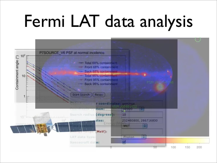
Fermi LAT data analysis PSR J0633+1746 VER J0648+152 4 0 50 100 150 200 Fermi Gamma-ray Space Telescope Large Area Telescope (LAT) ~20 MeV to >300 GeV Credit: NASA E/PO, Sonoma State University, Aurore Simonnet FOV: 2.4 sr
50 100 150 200
4 VER J0648+152 PSR J0633+1746
✦ ~20 MeV to >300 GeV ✦ FOV: 2.4 sr
✦ ~10 keV to ~25 MeV ✦ FOV: >8 sr
Credit: NASA E/PO, Sonoma State University, Aurore Simonnet
sightseers; guide’”
documentation/Cicerone/
target source
circular region centered at the target source start and end times
default: 100 MeV - 300 GeV
The region of interest (ROI) selection later on should be no bigger than this. Plan ahead or you have to download the data again!
ROI Time range Energy range
Event class (hidden!)
“INDEF” allows the parameters to be read from the header keywords
(Associated with the previous Pass6 IRFs) zenith cone buffer region
data is good
“Yes”: excludes time intervals where the buffer region intersects with the ROI
specify that you are making a counts map
dimensions of the counts map
50 100 150 200
4 VER J0648+152 PSR J0633+1746
To get the model which best describes the data, we wish to maximize L. In other words, we wish to find out the set of model parameters such that L is maximized.
Suppose the data is binned according to their positions in the sky and their energies. The number of counts in each bin is characterized by the Poisson distribution. The probability of detecting ni photons in the i-th bin is given by: where mi is the number of predicted photons by the model in that bin. The likelihood function L is defined as the product of the probabilities:
If we let the size of each bin to be infinitesimally small, then ni will be 0 or 1.
is the total number of predicted photons.
To make life simpler, we deal with the logarithm:
Good for small data sets (short observation time)
The Test Statistic (TS) is defined as (“likelihood-ratio test”): where Lmax,0 = the maximum likelihood value for a model without an additional source (the ‘null hypothesis’) Lmax,1 = the maximum likelihood value for a model with the additional source at a specified location Wilk’s Theorem: If the number of photons is sufficiently large, the TS for the null hypothesis is distributed like a χ2ν distribution, where ν is the difference in the number of parameters between the models with and without the additional source. Detection significance
“describes the gamma-ray sources in the sky (spatially + spectrally)” Source Model
spectral model e.g. simple power law, power law with exponential cutoff
isotropic all-sky (extra- galactic) emission
“templates”)
: position in the sky
In ordinary analysis, we treat as .
The model is folded with the instrumental response functions (IRFs) to obtain the number of predicted counts in the measured quantity space:
Effective area Energy dispersion PSF
http://www.slac.stanford.edu/exp/glast/groups/canda/lat_Performance.htm http://arxiv.org/abs/1206.1896
The likelihood will be evaluated many times during model fitting. To save CPU time, an “exposure map (cube)” is computed in advance (integral of total response over ROI data-space): which is independent of the source model. The log-likelihood becomes: where
Exposure map: total exposure for a given position in the sky producing counts in the ROI Pre-requisite: the time that a given position in the sky is observed at a given inclination angle (this is called the “livetime”) has to be known
This “livetime (exposure) cube” quantity is pre-computed by the tool gtltcube.
specifies the grid of the “livetime cube” specifies the grid of the exposure map the livetime cube is used as an input to compute the exposure map
e.g. pulsars e.g. blazars
The LAT 2-year Point Source Catalog is based
'myLATxmlmodel.xml')
'iso_p7v6source.txt', 'iso_p7v6source', ‘Templates’)
... ... $FERMI_DIR/refdata/fermi/galdiffuse/gal_2yearp7v6_v0.fits $FERMI_DIR/refdata/fermi/galdiffuse/isotropic_iem_v02_P6_V11_DIFFUSE.txt
Example use:
match the names!
(1) spectral part (2) spatial part [
Galactic diffuse and isotropic all-sky emission
Point-source: S is a delta-function, the integral is relatively easy Diffuse source: the integral is computational-intensive
Input source model, to determine: (1) whether pre-computed diffuse responses are present (2) whether an extended source is present in the model IRFs to use
“In the likelihood calculations, it is assumed that the spatial and spectral parts of a source model factor in such a way that the integral over spatial distribution of a source can be performed independently of the spectral part...”
keep your results! (for reference and for further iterations) we are performing unbinned likelihood analysis
in general: (1) DRMNFB (2) NEWMINUIT
store the screen
“[command] >& [file]”
dimensions of the
Goal: to find sources that are barely detectable. Model the strong, known, well- identified sources
not present in the model Moving a putative point source through a grid of locations in the sky and maximizing -log(likelihood).
40000 60000 80000 100000 120000