
SLIDE 1
ICC Module Computation Lesson 2 – Computation & Algorithms II
1
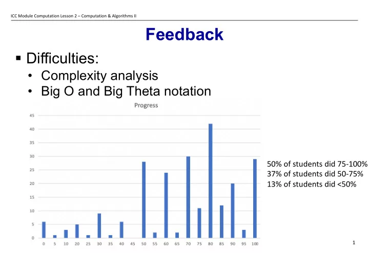
§ Difficulties:
- Complexity analysis
- Big O and Big Theta notation
Feedback Difficulties: Complexity analysis Big O and Big Theta - - PowerPoint PPT Presentation
ICC Module Computation Lesson 2 Computation & Algorithms II Feedback Difficulties: Complexity analysis Big O and Big Theta notation 50% of students did 75-100% 37% of students did 50-75% 13% of students did <50% 1 ICC
ICC Module Computation Lesson 2 – Computation & Algorithms II
1
ICC Module Computation Lesson 2 – Computation & Algorithms II
2
ICC Module Computation Lesson 2 – Computation & Algorithms II
3
ICC Module Computation Lesson 2 – Computation & Algorithms II
5
Algo1({5,8,6,10,3}) Algo1({8,6,10,3}) Algo1({6,10,3})
Algo1({10,3}) Algo1({3}) Algo1({})
ICC Module Computation Lesson 2 – Computation & Algorithms II
6
ICC Module Computation Lesson 2 – Computation & Algorithms II
7
ICC Module Computation Lesson 2 – Computation & Algorithms II
8
ICC Module Computation Lesson 2 – Computation & Algorithms II
10
rec_max({5,8,6,10,3}) rec_max({8,6,10,3}) rec_max({6,10,3})
rec_max({10,3}) Rec_max({3})
ICC Module Computation Lesson 2 – Computation & Algorithms II
11
ICC Module Computation Lesson 2 – Computation & Algorithms II
12
Month 1: 1 Month 2: 1 Month 3: 2 Month 4: 3 Month 5: 5 Month 6: 8
ICC Module Computation Lesson 2 – Computation & Algorithms II
13
In these pictures there are 55 curves of seeds spiraling to the left as you go outwards and 34 spirals of seeds spiraling to the right. A little further towards the center you can count 34 spirals to the left and 21 spirals to the right. These pairs of numbers are (almost always) neighbors in the Fibonacci series.
1 1 2 3 5 8 13
ICC Module Computation Lesson 2 – Computation & Algorithms II
14
F(5) = F(4)+F(3) F(4) = F(3)+F(2) F(3) = F(2)+F(1) F(3) = F(2)+F(1) F(2) = F(1)+F(0) F(2) = F(1)+F(0) F(1) F(2) = F(1)+F(0) F(1) F(1) F(0) F(1) F(0) F(1) F(0)
> "
!"# $%& ' 2! = 2 $(& ' − 1 = Ω(2 $ ')
< "
!"# $
2! = 2$%& − 1 = 𝑃(2$)
ICC Module Computation Lesson 2 – Computation & Algorithms II
15
ICC Module Computation Lesson 2 – Computation & Algorithms II
16
ICC Module Computation Lesson 2 – Computation & Algorithms II
17
ICC Module Computation Lesson 2 – Computation & Algorithms II
19
D (k,j)
k-1
Dk-1(i,j) D (i,k)
k-1
Zürich j Biel k-1 i Lausanne k Bern
ICC Module Computation Lesson 2 – Computation & Algorithms II
20
ICC Module Computation Lesson 2 – Computation & Algorithms II
21
(fictitious data)
ICC Module Computation Lesson 2 – Computation & Algorithms II
22
(fictitious data)
ICC Module Computation Lesson 2 – Computation & Algorithms II
23
(fictitious data)
ICC Module Computation Lesson 2 – Computation & Algorithms II
25
ICC Module Computation Lesson 2 – Computation & Algorithms II
26
ICC Module Computation Lesson 2 – Computation & Algorithms II
27
ICC Module Computation Lesson 2 – Computation & Algorithms II
28