
SLIDE 1
1
1
Feature Detection and Matching
Goal: Develop matching procedures that can detect
possibly partially-occluded objects or features specified as patterns of intensity values, and are invariant to position,
- rientation, scale, and intensity change
Template matching
gray level correlation edge correlation
Hough Transform Chamfer Matching
2
Applications
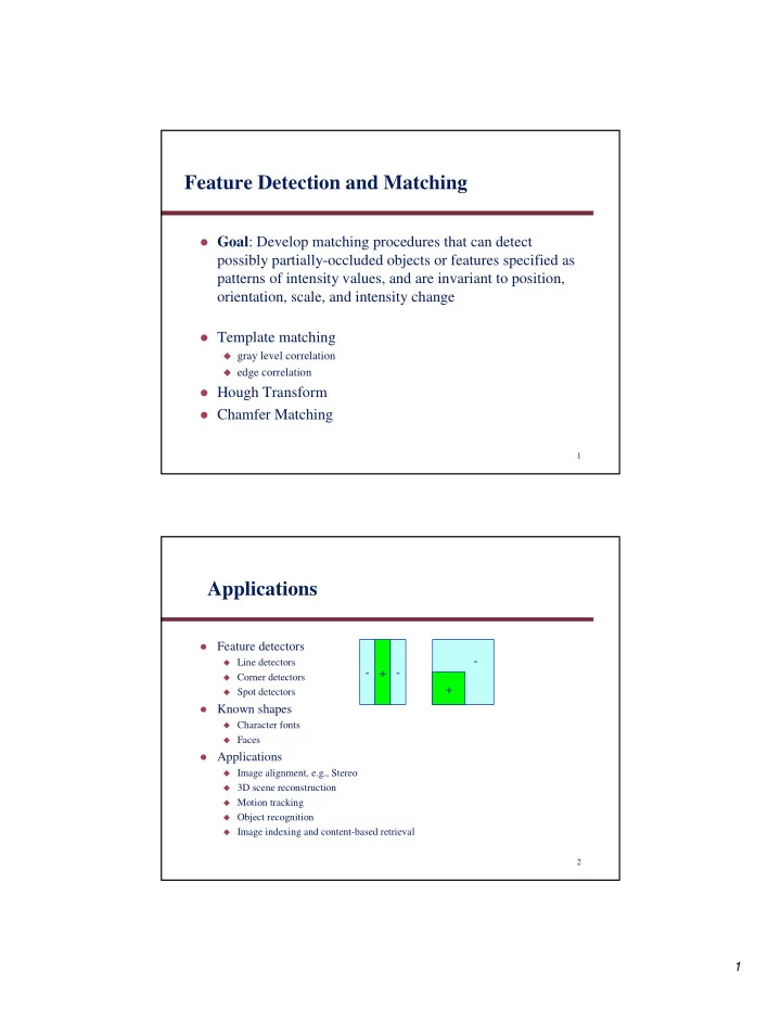
Feature detectors
Line detectors Corner detectors Spot detectors
Known shapes
Character fonts Faces
Applications
Image alignment, e.g., Stereo 3D scene reconstruction Motion tracking Object recognition Image indexing and content-based retrieval
- + -
+