FAST ALGORITHMS FOR THE COMPUTATION OF FOURIER EXTENSIONS OF - - PDF document

SLIDE 1

FAST ALGORITHMS FOR THE COMPUTATION OF FOURIER EXTENSIONS OF ARBITRARY LENGTH

ROEL MATTHYSEN, DAAN HUYBRECHS Abstract. Fourier series of smooth, non-periodic functions on [−1, 1] are known to exhibit the Gibbs phenomenon, and exhibit

• verall slow convergence. One way of overcoming these problems is by using a Fourier series on a larger domain, say

[−T, T] with T > 1, a technique called Fourier extension or Fourier continuation. When constructed as the discrete least squares minimizer in equidistant points, the Fourier extension for analytic functions has been shown shown to converge at least superalgebraically in the truncation parameter N. A fast O(N log2 N) algorithm has been described to compute Fourier extensions for the case where T = 2, compared to O(N3) for solving the dense discrete least squares

• problem. We present two O(N log2 N) algorithms for the computation of these approximations for the case of general

T, made possible by exploiting the connection between Fourier extensions and Prolate Spheroidal Wave theory. The first algorithm is based on the explicit computation of so-called periodic discrete prolate spheroidal sequences, while the second algorithm is purely algebraic and only implicitly based on the theory.

• 1. Introduction. Fourier series are a good choice for the approximation of a smooth periodic

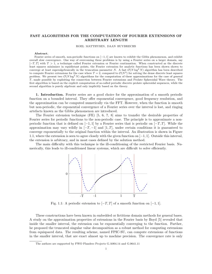
function on a bounded interval. They offer exponential convergence, good frequency resolution, and the approximation can be computed numerically via the FFT. However, when the function is smooth but non-periodic, the exponential convergence of a Fourier series over the interval is lost, and ringing artefacts known as the Gibbs phenomenon are introduced. The Fourier extension technique (FE) [5, 6, 7, 8] aims to transfer the desirable properties of Fourier series for periodic functions to the non-periodic case. The principle is to approximate a non- periodic function that is defined on [1, 1] by a Fourier series that is periodic on [T, T]. While the approximation may vary wildly in [T, 1[ and ]1, T], under certain conditions it is guaranteed to converge exponentially to the original function within the interval. An illustration is shown in Figure 1.1, where the extension is seen to agree closely with the given function on [1, 1]. Outside this interval, the extension is arbitrary, and in most cases defined by the solution method. The main difficulty with this technique is the ill-conditioning of the restricted Fourier basis. Nu- merically, this leads to ill-conditioned linear systems, which are difficult to solve efficiently.

• T
• 1

1 T

• Fig. 1.1: A periodic extension to [T, T] of a smooth function on [1, 1].

These constructions have been known in embedded or fictitious domain methods for general bases. A study on the approximation properties of extensions in the Fourier basis by Boyd [5] revealed that inside the smaller interval, the extension can be exponentially converging to the function. Further, he proposed the truncated singular value decomposition as a robust method for computing extensions from equispaced data. The resulting scheme, named FPIC-SU, can compute extensions of functions in the smaller interval, that are exact almost up to machine precision. The convergence rate is only

The authors are supported by FWO Flanders Projects G.A004.14 and G.0641.11 1

SLIDE 2

limited by the smoothness of the function. Bruno et. al. used the same principle when approximating surfaces by Fourier series on extended domains[7]. This provided a starting point for the very efficient FC-Gram method [9, 25, 4]. Exponential error convergence of the FE problem was proven in [18] when inverting the Grammian matrix of the continuous least squares problem. Later, Adcock et. al extended the convergence analysis to the discrete least squares problem on equispaced data. At least superalgebraic convergence was proven for analytic functions, when using the truncated SVD [2]. From an implementation point of view, the cost of the full SVD required for the FPIC-SU is prohibitively large. Recently, an FE algorithm was introduced by Lyon [23] that computes extensions in O(N log2 N) time. However, this algorithm only produces extensions of double length, i. e. it is unique to the case T = 2. Due to the reliance on symmetries only present when T is a power of 2, the algorithm cannot easily be extended to arbitrary T. In this paper we present fast algorithms for the computation of Fourier extensions of arbitrary extension length. One argument for varying the parameter T is found in the resolution power of the extension. The number of degrees of freedom per wavelength to represent an oscillatory function approaches the optimal value of 2 as T approaches 1 from above [1]. When T = 2, that number has already doubled. Other arguments may be performance related, as one may for example tune the length of the FFTs that are used in the computations, or a restriction on the data may be found in the application itself. Our algorithms stem from connecting the FE problem with classical results from signal processing

• theory. We state how it is essentially equivalent to the problem of bandlimited extrapolation. Central

in this discussion are the so-called Prolate Spheroidal Wave functions, originally introduced at Bell labs in the 1970s [30, 21, 22]. The study of these functions and their special properties has been an active domain in signal processing since. The connection with Prolate Spheroidal Wave theory leads to explicit formulations for eigenvectors

• f the FE problem. Analysis of the FE problem learns that the relevant ill-conditioning can be captured

using just O(log N) of these vectors. Combined with a fast solver for the remaining well-conditioned problem this leads to O(N log2 N) solvers. We explore two approaches in detail. In the first approach, a set of O(log N) discrete prolate spheroidal sequences is explicitly computed. This is based on their known properties: the vectors are known to be eigenvectors of a tridiagonal matrix. The second approach is purely algebraic and is not explicitly based on prolate spheroidal wave theory. Hence, this approach is more generally applicable. Both approaches have comparable performance, with a slight edge for the first approach. 1.1. Overview of the paper. We formally state the FE problem in §2 and summarize relevant previous results. A concise overview of Prolate Spheroidal Wave functions is presented in §3, including subsequent work on discrete variants. The connection between these discrete variants and the FE problem is used to obtain fast algorithms in §4. Finally, we present numerical experiments to illustrate the numerical performance of these algorithms in §5.

• 2. Fourier extensions.

2.1. Problem formulation. For the remainder of this paper we will focus on infinitely differ- entiable non-periodic functions f on the interval [1, 1]. Other intervals are easily dealt with through affine transformations. The approximation is constructed on the extended interval [T, T], with T the extension param-

• eter. For ease of notation denote

k(x) = 1 p 2T ei kπ

T x.

Then GN = {k}k=n,...,n

2

SLIDE 3

is the set of N = 2n + 1 Fourier basis functions on the extended interval. The Fourier extension problem is now formalised as finding an approximation FN(f) such that FN(f) = min

g2GN ||f g||[1,1].

(2.1) We note that the infinite set G1 is a basis for L2 on the extended interval [T, T], but it constitutes a frame on [1, 1] [12], i.e. it is redundant. This reflects the fact that a function can be extended in different ways. Once truncated to finite N, GN is actually a basis on [1, 1], albeit a very ill-conditioned

• ne. We refer to [2] for a detailed discussion of this point of view.

In an implementation context, it is more natural to consider the search for the Fourier coefficients a 2 CN, a = min

c2CN ||f n

X

k=n

ckk||[1,1]. Depending on the norm to be minimised, the extension problem takes on a different formulation: Discrete Fourier extensions. Most practical applications provide information about f as samples in a predefined set of points. The norm in (2.1) is then conveniently replaced by a discrete least squares norm ˜ FN(f) = min

g2GN

X

l

(f(xl) g(xl))2 , xl 2 [1, 1]. (2.2) Previous work distinguishes between uniform sampling, and an optimal sampling set called mapped symmetric Chebychev nodes [1]. The focus of this paper is on the case where the sampling points are uniform, xl = l m, l = m, . . . , m, for a total of M = 2m + 1 points. Typically, some oversampling is used so M = N > N. Including appropriate normalisation, this leads to the matrix formulation that is used throughout the rest of the

• paper. Let

Al,k = k(xl) = 1 p 2Tm ei πkl

T m ,

bl = 1 pmf(xl), l = m, . . . , m, k = n, . . . , n. (2.3) Note that matrix-vector products involving A can be performed very efficiently using FFTs of length L = 2Tm. Therefore L is assumed to be integer for the remainder of this paper. The Fourier coefficients are then found by collocation, through solving the rectangular system Aa ⇡ b (2.4) in a least squares sense. Note that due to the nature of the problem we are not interested in a specific solution a, just one of the possibly many solutions that lead to a small residual ||Aa b||. Solving this problem efficiently is the focal point of this paper. Continuous Fourier extensions. When the norm is the regular L2-norm over [1, 1], F N(f) = min

g2GN ||f g||2,[1,1]

is known as the continuous Fourier extension. The resulting least-squares problem can be solved by formulating the Grammian matrix. Let ¯ Ai,j = Z 1

1

i(x)j(x)dx = sin π(ij)

T

⇡(i j) , bi = Z 1

1

fi(x)dx, i, j = n, . . . , n. (2.5) Then the Fourier coefficients follow from ¯ Aa = b. (2.6)

3

SLIDE 4

2.2. Convergence and stability. The usefulness of approximation schemes hinges on two prop- erties: the speed of convergence to the given function, and the stability of the required computations. Considerable effort has been put into quantifying these properties both analytically and numerically [18] [1] [2] [24]. Without going into too much detail, we recap the most important results. First of all, a distinction should be made between the exact discrete and continuous FE solutions ˜ FN(f) and F N(f), and their computer-implemented counterparts. Computing the exact solutions is known to be unstable, as they can grow unbounded outside the interval of interest. Numerical algorithms however will never compute these exact solutions. Due to regularisation, the numerical FEs ˜ GN(f) and GN(f) are more stable, while maintaining the desired convergence behaviour. In [2], the truncated SVD was used as a model scheme for solving the ill-conditioned systems (2.3) and (2.5). Given the Singular Value Decomposition of the FE matrix A = USV 0, the solution to Aa = b is a = V S†U 0b, S†

i,i =

(

1 Si,i

Si,i > ⌧

• therwise.

(2.7) The truncation parameter ⌧ then acts as a regularisation parameter. It is usually chosen close to the machine precision.

• Stability. Following [2], stability is defined in terms of the absolute condition number of the FE

mapping (FN) = sup{||FN(b)|| : b 2 CN, ||b|| = 1}, where, with slight abuse of notation, FN(b) is the solution to the FE problem with right hand side b, and ||·|| is the regular l2 norm over [1, 1]. This condition number can be computed for the continuous and discrete FEs, both the exact and numerical versions. It was shown to grow exponentially in N for the exact solution to the continuous and discrete FE problem. When looking at the numerical FEs the situation changes considerably. The condition number

• f the numerical continuous FE mapping is (GN) . 1/p⌧. The condition number of the numerical

discrete FE ( ˜ GN) is dependent on a constant 0 < a(; T)  1, independent of N, that satisfies a(; T) ! 0 as ! 1 for fixed T. It is given by ( ˜ GN) . ⌧ a(γ;T ), 8N 2 N. This means that for a sufficiently large oversampling factor , the condition number of the numerical FE mapping can be made reasonably close to 1. Meanwhile, the condition number of the matrices A and ¯ A grows exponentially as N ! 1, where M N for the discrete FE. This is surprising, given the good condition of the FE mapping. It can be understood by noting that extensions with small coefficient norm and small residual are guaranteed to exist. The numerical algorithms will steer clear of the unstable exact solution, and instead return

• ne of these alternatives. For a full exposition on the stability of FE calculations, see [2].
• Convergence. Concerning convergence, results in [2] are valuable only for functions that are ana-

lytic in a region D(⇢⇤) of the complex plane and continuous on its border. This region is a Bernstein ellipse under a transformation that allows Fourier extensions to be understood as polynomial approx-

• imations. For such functions f, the exact continuous and discrete FEs converge geometrically, with a

speed ||f ˜ FN(f)||  cf⇢N. Here ⇢ = min{⇢⇤, E(T)} and cf is proportional to maxx2D(ρ) |f(x)|. E(T) is known as the Fourier extension constant and is given by cot2 π

4T

• . Note that for the exact discrete FE, there is an added

requirement of scaling M as O(N 2), to avoid the Runge phenomenon. Under the same analyticity conditions, the error decay of the numerical counterparts GN and ˜ GN can be broken down into several subregions:

• 1. If N < N2, where N2 is a function-independent breakpoint, ||f ˜

GN(f)|| converges or diverges exponentially fast at the same rate as the exact solution.

4

SLIDE 5

• 2. When N  N0 (continuous) or N2  N  N1 := 2N0 (discrete), where N0 is another function-

independent breakpoint depending, both ||f GN(f)|| and ||f ˜ GN(f)|| decay like ⇢N.

• 3. When N = N0 or N = N1, the errors are approximately

||f GN0(f)|| ⇡ cf(p⌧)df , ||f ˜ GN1(f)|| ⇡ cf⌧ df a(γ;T ), where cf is as before, and df =

log ρ log E(T ) 2 (0, 1].

• 4. When N > N0 or N > N1, the errors decay at least super algebraically fast down to maximal

achievable accuracies of order p⌧ and ⌧ 1a(γ;T ) respectively. This behaviour of the error offers insight into the usability of Fourier extensions. A first observation is that the continuous FE is limited to a maximal achievable accuracy of p⌧. Coupled with the need to compute Fourier integrals to compose the right hand side b in (2.5), this makes the continuous FE unfit for practical use. However, the algorithms presented in §4 for the discrete FE can be adapted to this context with little extra effort. This is documented in §4.3. On the contrary, the numerical discrete FE guarantees convergence up to a certain power of ⌧. By varying this cutoff, the oversampling and the extension length T this maximum achievable accuracy can be made very close to the machine precision. 2.3. Influence of the extension length. The main contributions of this paper are algorithms that add flexibility in the choice of extension length T. The increased resolution power was already cited as an argument to reduce T, but it is important to be aware of the possible consequences. Therefore, in this section we summarize the influence of this parameter on convergence, resolution power, and conditioning of the FE problem. First note that the Fourier extension constant E(T) grows with T. For functions analytic in a sufficiently large region, the convergence rate ⇢ is limited by this constant. Increasing T thus increases the convergence rate, and vice versa. The resolution power of a scheme, first studied by Gottlieb and Orszag [15] is a measure of the amount of point samples needed to resolve an oscillatory function to a certain precision. Let R(!, ) = min{N 2 N : ||eiπω FN(eiπω)||1 < }, ! > 0, for some small . Then FN has a resolution constant r if R(!, ) ⇠ r!, ! ! 1. For regular Fourier series, this constant has the optimal value 2. A theoretical argument shows that for the continuous FE this resolution constant increases with T [1]. More specifically, r(T)  2T sin ⇣ ⇡ 2T ⌘ , T 2 (1, 1). Thus, for T ⇡ 1 the resolution constant r(t) ⇡ 2T is close to optimal. When T tends to infinity, r(T) ⇠ ⇡. It is even possible to optimally balance convergence speed with resolution power when aiming for a predetermined accuracy ✏tol. This is achieved by varying T with N, specifically T(N, ✏tol) = ⇡ 4 ⇣ arctan(✏tol)

1 2N

⌘1 . (2.8) Although no equivalent analysis exists for the discrete FE, there have been several attempts to determine FE parameters that are in some sense optimal. In [8], Bruno et. al. suggest the values T = 2 and = 2 as a general rule of thumb, but at the same time notes that the optimal parameters are heavily function dependent. Note that increasing both the extension length T and the oversampling will likely increase the resolution constant r. Especially since it was shown in [1] that the limit r(T) ⇠ ⇡ as T ! 1 no longer holds for a discretised FE, instead the resolution constant grows as

5

SLIDE 6

r(T) ⇠ 2T. Even though this was only observed for data points distributed as a variant of Chebychev points, it is indicative that the resolution constant for T = 2, = 2 will be considerably above the

• ptimal value.

The precise interplay between T and on the one hand, and resolution power and conditioning on the other hand was studied in detail by Adcock and Rua [3]. They found that the condition number ( ˜ GN) of the equispaced discrete FE depends only on the product T. Increasing either will lower the condition number. Thus as long as is increased or decreased accordingly when varying T, the conditioning of the FE mapping remains constant. This is cited as an argument to limit T to 2, to profit from the at the time only available fast FE algorithm. Furthermore, the resolution constant is also dependent on the product T, growing as r(T) ⇠ T. This illustrates the tradeoff between resolution power and conditioning. Numerical experiments in [3] showed that by allowing the condition number to grow from  ⇡ 10 to  ⇡ 100, the resolution constant was halved, while further increasing  had very little additional value. However, it should be noted that these experiments were only carried out for T = 2. Lifting the restriction on T may thus offer more flexibility in finding a balance between resolution power and conditioning. An interesting open problem raised in [3] is the possibility to vary T with M, to achieve optimal resolution power in a manner similar to (2.8). Due to the lack of a fast algorithm, any gains from varying T were considered of limited practical usability compared to the fast algorithm for T = 2. The fast algorithms presented in this paper warrant a closer look at the possible benefits from this method. Remark 1. The fast algorithms in this paper all depend on the application of the FFT, requiring L = T(M 1) to be integer. Strictly speaking, this means that T is restricted to be a rational number and, hence, T is not completely arbitrary. Furthermore, in applications where the number of function samples M is fixed in advance, T can only vary in increments of 1/(M 1). For large M, the latter restriction is not very limiting. The restriction to a rational number, say T = p/q, means that the methods will be more practical if the denominator q is not too large, since large q would necessitate large values of L and M.

• 3. Prolate spheroidal wave functions and discrete variants. A long-standing problem in

signal processing theory is that of bandlimited extrapolation. The problem is, assuming some portion

• f a bandlimited signal is known, to accurately predict the missing data. In a first subsection we explain

how the FE problem is a specific variant of this problem. The subsequent sections then explore the theory of Prolate Spheroidal Wave functions, that plays a major role in bandlimited extrapolation, for further use in the FE algorithms. 3.1. Discrete Fourier extensions and bandlimited extrapolation. The discrete Fourier extension is closely related to discrete band limited extrapolation, i.e., to the problem of reconstructing a discrete bandlimited signal from a number of data samples. Simply put, we are looking for a vector y with discrete Fourier transform Y such that y[k] ⇡ f[k] k 2 SM,t Y [l] = 0 l 62 SN,ω, where f is the sample data, and SM,t and SN,ω are sampling sets in the discrete time and frequency domains, of sizes M and N respectively. Depending on the problem parameters the solution might not be unique. In this case an additional minimal solution norm constraint can be added [19]. A popular method is the Papoulis-Gerschberg algorithm [14] [26]. It uses a two-step iteration process to alternate matching the given data and complying with the frequency constraints. Variants that use the conjugate gradients and related methods to speed up the iteration process tend to perform reasonably well numerically [31]. They operate at a cost of O(N log N) operations per iteration, where the number of iterations scales with the bandwidth of the signal. Besides these iterative methods, considerable attention was given to direct methods for solving this discrete problem. One such method is the one proposed by Jain and Ranganath [19], where both the time and frequency sampling sets are contiguous, i. e. St = m, . . . , m and Sω = n, . . . , n. They

6

SLIDE 7

commence by writing the data as a function of the unknown coefficients: f = Jy = DMBNy (3.1) DM,i,j = i,j, |i|, |j|  m (3.2) BN,p,l = 1 L

n

X

k=n

exp i(p l)2⇡k L = 1 L sin ⇣

(pl)Nπ L

⌘ sin ⇣

(pl)π L

⌘ . (3.3) Here, BN is a L ⇥ L circulant matrix that represents a discrete low-pass filter, and DM is a M ⇥ L selection operator. i,j is the kronecker delta. D0

M is an extension operator that pads a sequence of

length M with zeros to length L. The direct methods of Jain and Ranganath then consist of solving Jy = f in a least squares sense by formulating the normal equations J0Jy = J0f. Since J0J is symmetric positive definite and Toeplitz, the Levinson-Trench algorithm can be applied to compute the inverse of J0J in O(L2) operations. They also suggested another approach, using the singular value decomposition of J to solve the least-squares problem. The resulting singular vectors were named periodic discrete prolate spheroidal sequences (P-DPSSs), after the prolate spheroidal wave functions (PSWFs) arising in continuous bandlimited extrapolation. A closer look at the matrix A from the discrete Fourier extension (2.3) makes the relation with (3.1) apparent. Adopting the notation for the DFT length L = 2Tm, (AA0)pq = 1 L

n

X

k=n

exp i(p q)2⇡k L , p, q = m, . . . , m = (DMBND0

M)pq = (JJ0)pq,

(3.4) where the last line follows from the idempotency of BN. Consequently, A and J share the same left singular vectors, and the same singular values. Essentially, discrete Fourier extension is a reformulation

• f the bandlimited extrapolation problem with the N frequency coefficients as unknowns, instead of

the extrapolated signal. The focus has also shifted from determining an accurate extension to the approximation of the given data samples. The next sections concern the PSWFs and P-DPSSs, and how they are natural solutions for the bandlimited extrapolation problem. The groundwork for this theory was detailed in a series of papers by Slepian, Landau and Pollak from 1961 onwards [30, 21, 22, 27, 28]. An overview is given in [29]. 3.2. Prolate Spheroidal Wave Functions. Denote by f(x) and F(⇠) a function in L2 and its Fourier transform, so that F(⇠) = Z 1

1

f(x)e2πixξds, f(x) = Z 1

1

F(⇠)e2πixξd⇠. The time- and bandlimiting operators D and B are then defined as Df(x) = ˆ f(x) = ( f(x) |x|  T |x| > T Bf(x) = Z Ω

Ω

F(⇠)ei2πξxd⇠, (3.5) which project onto L2

[T,T ] and PWΩ, the Paley-Wiener space of bandlimited functions, respectively.

Note that the bandlimiting operator can also be written as Bf(x) = Z 1

1

f(s)sin(2⇡Ω(x s)) ⇡(x s) ds.

7

SLIDE 8

The Heisenberg-Gabor limit states that no nonzero function can be simultaneously concentrated in both time and frequency, and so 8f 6= 0 : ||BDf|| < ||f||. However, one can look for nearly-invariant functions under this operator, functions for which ||BDf||/||f|| is as close to 1 as possible. These are the eigenfunctions of the operator BD, i. e. the solutions of the integral equation (x) = Z T

T

(s)sin(2⇡Ω(x s)) ⇡(x s) ds. (3.6) Slepian and collaborators showed that this equation is solvable only for select values of , a countably infinite set 1 > 0 > 1 > · · · > 0. The corresponding eigenfunctions i were named Prolate Spheroidal Wave functions. The naming stems from the curious observation that these functions are solutions to the spheroidal wave equation ✓ 1 x2 T 2 ◆ d2 i dx2 2xd i dx (2⇡ΩT)2 x2 i = ✓i i. (3.7) This is a Sturm-Liouville equation with a set of unique eigenvalues · · · > ✓i1 > ✓i > ✓i+1 > . . . corresponding to the functions i[30]. Since B and D are idempotent operators, it is convenient to consider the i eigenfunctions of the Hermitian operator BDB. Timelimiting both sides of (3.6), the timelimited functions ˆ i = D i are the eigenfunctions of the Hermitian operator DBD, with corresponding eigenvalues i. The term Prolate Spheroidal Wave function is used for both the i and the ˆ i. As eigenfunctions of a Hermitian operator, the i and ˆ i are orthogonal Z 1

1

i(x) j(x)dx = ij Z T

T

ˆ i(x) ˆ j(x)dx = iij, and they are complete in PWΩ and L2

[T,T ], respectively. The Prolate Spheroidal Wave functions

thus form an orthogonal base for PWΩ, and the eigenvalue i represents the fraction of energy of i contained in [T, T]. This leads to a straightforward approach to continuous bandlimited extrapolation. Let f be a function segment in L2

[T,T ]. Then

g = X

i

1 i h ˆ i, fi[T,T ] i (3.8) is a bandlimited function that agrees with f in the interval due to the completeness of the ˆ i in L2

[T,T ].

Furthermore, when truncating the sum, the first terms have the largest eigenvalues and capture the most energy inside the interval. Using both (3.6) and (3.7), the PSWFs were further shown to have the following properties [30]: i The i are eigenfunctions of the finite Fourier transform, Z T

T

ei2πtξ n(t)dt = in ✓T Ω ◆1/2 n ✓⇠T Ω ◆ . ii The eigenvalues i cluster near 1 for low values of i, and decay exponentially after a set breakpoint i ⇡ 1, i ⌧ 4ΩT and i ⇡ 0, i 4ΩT. The width of the region where i 2 (✏, 1 ✏) grows as log(ΩT). The first property illustrates the symmetry of time and frequency domain in this problem. The second property shows that a truncated approximation (3.8) will require ⇡ 4ΩT terms. The increasing irregularity of the ˆ i coupled with the exponential decay of the i ensures that g will converge rapidly after this breakpoint for a sufficiently regular f.

8

SLIDE 9

3.3. Periodic Discrete Prolate Spheroidal Sequences. There are several possible discreti- sations for PSWFs. The most well-known is the one proposed by Slepian, where the Fourier transform is replaced with the discrete-time Fourier transform G(f) =

1

X

n=1

g[n]ei2πfn, g[n] = 1 2⇡ Z 1/2

1/2

G(f)ei2πfnd f. The resulting generalisations are frequency domain functions on [1/2, 1/2] commonly referred to as discrete prolate spheroidal wave functions (DPSWFs), and infinite sequences in the time domain called discrete prolate spheroidal sequences (DPSSs). The properties from section 3.2 carry over, apart from some loss of symmetry between time and frequency domains [28]. Another approach was proposed independently by Jain and Ranganath [19] and Gr¨ unbaum [17], and elaborated on in [33]. They replace the Fourier transform with the DFT for sequences of length L: Hk =

L1

X

n=0

h[n]ei2πkn/L h[n] = 1 L

L1

X

k=0

Hkei2πkn/L. The discrete analogues of the time- and bandlimiting operators are given by the matrices (3.2) and (3.3) from the discrete band limited extrapolation problem. Similar to the continuous PSWFs, the periodic discrete prolate spheroidal sequences (P-DPSS) i are defined as the eigenvectors of the hermitian matrix operator BND0

MDMBN, and their limited versions ˆ

i as the eigenvectors of DMBNDM BND0

MDMBNi = ii

DMBND0

M ˆ

i = i ˆ i. (3.9) Since DMBND0

M is not of full rank when M > N, an additional requirement that i 6= 0 is imposed,

following [33]. Consequently, there are only {min(N, M)} P-DPSSs. The i properties are similar to those of PSWFs: i If M N, the i are complete in the space of bandlimited sequences spanned by BN. ii If M  N, the ˆ i are complete in RM. iii The i are doubly orthogonal i · j = ij, Di · Dj = iij iv The P-DPSSs are eigenvectors of the finite DFT, but with the roles of M and N interchanged DNFM,N,i = ˆ N,M,i. Here, F is the DFT matrix of size L. v Among sequences of length L, with frequency support in [0, m] [ [L m, L], 0 is the most con- centrated in [0, M 1]. Among sequences of equally limited frequency support orthogonal to 0, 1 is the most concentrated in [0, M 1], and so on. vi Like the eigenvalues of the PSWFs, the eigenvalues i are distinct and cluster exponentially near 1 and 0, in that i ⇡ 1, i ⌧ NM L and i ⇡ 0, i NM L . The width of the plunge region where i 2 (✏, 1 ✏) grows as log(NM/L) [32]. vii The P-DPSSs satisfy a second order difference equation [33] bk ˆ i[k 1] + ck ˆ i[k] + bk+1 ˆ i[k + 1] = ✓i ˆ i[k], k = 0, . . . , M 1, (3.10) with coefficients bk = sin ✓⇡k L ◆ sin ✓⇡(M k) L ◆ ck = cos ✓⇡(2k + 1 M) L ◆ cos ✓⇡N L ◆ .

9

SLIDE 10

Equation (3.9) clarifies their importance in both the discrete band limited extrapolation problem, and discrete Fourier extensions. From (3.4) it is obvious that the eigenvectors of AA0 and JJ0 are the limited P-DPSSs ˆ

• i. Regarding the singular value decompositions of A and J, this determines the left

singular vectors as ˆ i and the associated singular values as pi. For J, following J0J = B0

ND0 MDMBN = BNDMBN,

the right singular vectors are seen to be full P-DPSSs i. Using these relations, Jains SVD method results in an extrapolated sequence g[n] =

N1

X

i=0

1 pi ⇣ ˆ i · f ⌘ i, similar to the continuous extrapolation (3.8). The discrete Fourier extension matrix A differs from J in the right singular vectors. Similar to (3.4) A0A = (

m

X

l=m

exp i(p q)2⇡k L ) , p, q = n, . . . , n = DNBMDN. The right singular vectors are then again limited P-DPSSs ˆ i, where the parameters N and M have been interchanged. Using ˆ Φ to represent the set of P-DPSSs and Υ for the diagonal matrix of eigen- values, the SVD of A is given by A = ˆ ΦM,N p Υˆ Φ0

N,M.

Calculating the coefficients of the discrete FE by truncating the SVD now corresponds to a =

ic

X

i=0

1 pi ⇣ ˆ N,M,i · f ⌘ ˆ M,N,i, where ic is determined by the cutoff parameter, pic ⌧ > pic+1. This formulation of the FE together with the P-DPSS properties listed above leads to the fast algo- rithms in the next section.

• 4. Algorithms. In this section we present two approaches to computing the truncated SVD

solution to the discrete Fourier extension problem Ax = b. Both approaches are based on a specific division in easier subproblems, which is explained below. They differ only in how they solve one of these subproblems. Detailed algorithms follow in sections 4.1 and 4.2. From the previous section, the SVD of the FE matrix A is A = UΣV 0 = ˆ ΦM,N p Υˆ Φ0

N,M.

The cost of this full SVD is prohibitively large, growing as O(N 3). To reach the performance goal

• f O(N log N) operations, two subproblems are identified and solved in succession. The key to this

division is in the distribution of the singular values Σ, as shown in figure 4.1. Three distinct regions are visible. Following property (vi) of the P-DPSS, they are for some small cutoff ⌧:

• A region Iα := { : 1 > > 1 ⌧} where all singular values are 1 up to a tolerance ⌧. This

region contains approximately O(NM/L) singular values.

10

SLIDE 11

N/T 1016 108 100 i i Iγ Iβ Iα

• Fig. 4.1: The subdivision of the spectrum of A into three distinct intervals, with cutoff parameter

⌧ = 1e 14. Due to rounding errors, the eigenvalues in region Iγ don’t decay past machine precision.

• A region Iβ := { : 1 ⌧ > ⌧}, also referred to as the “plunge region” in a more general

context regarding truncated frames. The number of singular values in this region grows as O(log (NM/L)).

• A region Iγ := { : ⌧ > 0} where the singular values further decay exponentially.

Let the subdivision of the singular values and associated vectors be denoted by A = ⇥Uα Uβ Uγ ⇤ 2 4 Σα Σβ Σγ 3 5 ⇥Vα Vβ Vγ ⇤0 . The truncated SVD solution to the problem Ax = b with truncation cutoff at ⌧ is then x = xα + xβ = VαΣ1

α U 0 αbα + VβΣ1 β U 0 βbβ,

(4.1) where the inverse operator applies to the diagonal elements. The right hand side is split along the

• rthogonal spans of Uα, Uβ and Uγ, i.e.,

bα = UαU 0

αb,

and so on. Note that this solution method implicitly assumes bγ to be below the required solution

• accuracy. If it is not, a large solution term xγ is needed, with ||xγ|| 1

τ ||bγ||. In this case, we say the

Fourier extension has not yet converged, and N should be increased. Equation (4.1) splits the problem into two orthogonal subproblems. The isolation of Vβ, Sβ and Uβ from the plunge region and efficient calculation of xβ is where the two approaches given in sections 4.1 and 4.2 differ. The subsequent calculation of xα is then straightforward, based on the following observation: A0(b bβ) = VαΣαU 0

αbα + VγΣγU 0 γbγ

= VαΣ1

α U 0 αbα + O(⌧)

= xα + O(⌧) The bγ term, which is already assumed to be negligible, is fully eliminated by the additional O(⌧) factor Σγ. Noting that Σα = Σ1

α + O(⌧) then yields xα at the cost of a single fast multiplication with

A0 (O(N log N)).

11

SLIDE 12

4.1. Approach 1: explicit projection onto prolate sequences. Due to the intrinsic connec- tion of the FE problem with DPSSs, it is possible to explicitly compute Uβ, Σβ and V 0

β. The second

• rder difference equation from (3.10) implies that

ZM,N ˆ M,N,i = ✓i ˆ M,N,i, ZM,N = 2 6 6 6 6 4 c0 b1 b1 c1 ... ... ... bN1 bN1 cN1 3 7 7 7 7 5 . (4.2) The P-DPSSs can thus be found as eigenvectors of a tridiagonal matrix. The ˆ M,N,i that make up U are eigenvectors of ZM,N. The dual matrix ZN,M yields the right singular vectors V . With the P-DPSSs known, the original singular value is found in O(N log N) operations as i = ˆ

m,n,iAˆ

n,m,i This approach is already in use for the regular DPSSs [16]. In this stage of the algorithm however, we are only interested in a subset of the singular values and vectors. Since the number of singular values in the plunge region is logarithmically small, we look to algorithms that calculate k eigenvalues and eigenvectors of a tridiagonal matrix Z in O(kN)

• perations [11]. Algorithms for this computation require as input for the desired eigenvalues ✓i of Z

either:

• A range [C1, C2]: the algorithm then finds all ✓ : C1  ✓  C2.
• A index set {imin, . . . , imax}: the algorithm then finds all ✓ : ✓imin  ✓  ✓imax, from the
• rdered set ✓0 ✓1 . . . .

The algorithms thus require knowing the ✓j, or alternatively the indices j, that correspond to i 2 Iβ. Denote the mappings between i and ✓j, and between their indices i and j, by ✓j = GN,M(i), j = G0

N,M(i) ,

(ˆ

iZN,M ˆ

i = ✓j ˆ

iAN,M ˆ

i = i. The description of GN,M(Iβ) is difficult, as very little is known of this mapping. The only known trait is monotonicity, a trait shared with the PSWF and DPSWF equivalents. This is already very helpful, since it implies that G0

N,M(i) = i.

Theorem 1. For M N, the mapping G0

N,M is monotone,

8i1, i2 : i1 > i2 , G0

N,M(i1) > G0 N,M(i2).

• Proof. The proof follows a mechanism used by Slepian in both [30, p. 61] and [28, §4.1]. The

continuity of eigenvalues and eigenvectors as a function of a parameter, combined with a known ordering result for a specific value of this parameter, extends the known result to all parameter values. First we recall a similar result from the continuous Fourier Extension. Let ¯ A be the matrix of the continuous FE (2.5) with eigenvalues ¯ i, and ¯ ZN the tridiagonal matrix (4.3) with eigenvalues ¯ ✓i ¯ ZN = 2 6 6 6 6 4 p¯ c0 ¯ b1 ¯ b1 ¯ c1 ... ... ... ¯ bN1 ¯ bN1 ¯ cN1 3 7 7 7 7 5 , ¯ ci = ✓N 1 2 i ◆2 cos ⇡ T , ¯ bi = i(N i) 2 . (4.3)

12

SLIDE 13

Then the mapping ¯ G0 j = ¯ G0(i) , (¯

i ¯

ZN ¯ i = ¯ ✓j ¯

i ¯

A¯ i = ¯ i , was proven to be monotone in [30, §4.1]. This result can be extended to the discrete FE case, since the limits of the entries of A0A and ZN,M for large m can be written in terms of the corresponding matrices of the continuous problem: lim

m!1(A0A)ij = sin (ij)π T

⇡(i j) = ¯ Aij lim

m!1 bk = ⇡2k(N k)

L2 = 2⇡2 L2 ¯ bk lim

m!1 ck = cos ⇡

T 2⇡2 L2 ✓N 1 2 k ◆2 1 ! = 2⇡2 L2 ¯ ck cos ⇡ T lim

m!1 ZM,N = 2⇡2

L2 ¯ ZN cos ⇡ T I The last line ensures that the eigenvalues of ZM,N are those of ¯ ZN under a linear mapping. Since this mapping preserves the ordering of eigenvalues, the theorem holds in the limit m ! 1. Further, when limited to the regime T > 1, 2m + 1 N, we have the following:

• 1. The tridiagonal matrix ZM,N(m) with diagonal elements ck and subdiagonal elements bk

bk = sin ✓ ⇡k 2Tm ◆ sin ✓⇡(2m + 1 k) 2Tm ◆ ck = cos ✓⇡(k m) Tm ◆ cos ✓ ⇡N 2Tm ◆ . commutes with A0A for integer values of m. However, by a substitution as in [10, Thm. 4.7], it is easy to see that this relationship holds for any real m > n.

• 2. A classical result states that the eigenvalues of a matrix are continuous as the matrix entries

vary continuously in the parameter. Thus all ✓i(m) are continuous. In general they may coincide with each other. However, since all subdiagonal entries are always non-zero, 81  k  N 1 : b2

k > 0,

ZM,N(m) is a so-called normal Jacobi matrix and such matrices are known to have distinct eigenvalues [13, Ch. 2.1]. As a result of this distinctness, the eigenvectors can be chosen to be continuous in m as well [20, Ch. 2 §5.3].

• 3. To prove similar statements for the matrix A0A, we note that the inductive proof in [33,
• Prop. 5] for the distinctness of eigenvalues of A0A is dependent only on it being symmetric,

and the commuting ZM,N(m) being a normal Jacobi matrix. The eigenvalues i(m) are thus continuous and distinct 8m n. Then the eigenvectors can also be chosen continuous in m. Combining these statements, the distinctness preserves the relative ordering of the continuous eigenval-

• ues. The continuity of the eigenvectors relates the eigenvalues of A and ZN,M through the mapping G0.

Since this mapping is monotone in the limit m ! 1, the continuity ensures the mapping is monotone for all m n. The required index set for the eigenvalues of ZM,N is exactly the index set corresponding to i from the plunge region. From (vi) these are known to be centered around NM

L , and their number

grows as O(log N). All that remains is to determine the constants Cmin and Cmax so that j 2 Iβ , j 2  max ⇢ N NM L Cmin log N, 1

• , min

⇢ N NM L + Cmax log N, N

• .

13

SLIDE 14

We denote the minimum and maximum indices as jmin and jmax. The minimum required index set [jmin, jmax] with cutoff ⌧ = 1e 16 for increasing N is shown in Figure 4.2, with the value N NM

L

as a dashed line. Experimentally, the choices Cmin 6 and Cmax 3 seem sufficient for all ⌧ ✏mach. The Vβ can be obtained by refining A0 ˆ M,N,i as eigenvectors of ZN,M. Using a fast tridiagonal eigenvector algorithm, Uβ, Σβ and Vβ can be computed in O(N log N)

• perations. The solution term

xβ = VβΣ1

β U 0 βb

is then found in O(N log2 N) operations. Remark 2. Monotonicity of the map GN,M is also observed to hold for integer M smaller than integer N. Specifically, a variant of Theorem 1 holds for the M nonzero singular values i. The same index set can thus be used to compute both Uβ and Vβ with a fast tridiagonal eigenvalue algorithm. However, this altered algorithm is without proof. 50 100 150 200 250 300 350 200 400 N [jmin, jmax] T=4/3 T=2 T=10/3

• Fig. 4.2: The behaviour of the index set of the plunge region. The minimal and maximal index of the

plunge region are shown as solid lines, for different values of T. The point NM/L, which is known to lie in the interval, is shown as a dashed line. Combining xβ with the calculation of xα described above leads to a fast O(N log2 N) algorithm. A bare-bones version incorporating remark 2 is given in Algorithm 1. The trideig function should return eigenvectors of a tridiagonal matrix given an index interval, e.g. the lapack routine dstevx. The matrix-vector multiplications with A and A0 should be implemented using a combination of length L unitary FFTs F and F 0 and selection matrices DM and DN: A = DMF 0D0

N

A0 = DNFD0

M.

Here, DN selects the subset of frequencies that correspond to the Fourier series approximation from the longer FFT, i.e., the 2N + 1 smallest frequencies. The matrix DM selects the function samples that lie in the approximation interval from the equispaced samples on the extended interval. We have used a symmetric embedding [1, 1] 2 [T, T] in this paper, but other choices are possible. We refer to the matlab implementation of these matrix-vector products in the appendix for the details of the implementation. 4.2. Approach 2: an implicit projection method. The second approach to calculating xβ is more universal, or more generally applicable, since it depends solely on the steep singular value profile discussed earlier and illustrated in Fig. 4.1. As such, it is extensible to any ill-conditioned basis that exhibits a similar profile.

14

SLIDE 15

Algorithm 1 Explicit projection on DPSSs Uβ =trideig(ZM,N, {jmin , jmax }) Vβ =trideig(ZN,M, {jmin , jmax }) Σβ = (U 0

βAVβ) > ⌧

xβ = VβΣ1

β U 0 βb

xα = A0(b Axβ) x = xα + xβ The approach is based on the observation that multiplying both the FE matrix A and right hand side by a factor P = (AA0 I) (4.4) isolates the problem to the plunge region. This is most easily seen from the SVD. With A = UΣV 0 we have P = U(Σ2 I)U 0, (4.5) and PA = U(Σ3 Σ)V 0. Note here that the mapping P() = 3 isolates the singular values from the plunge region since 8 2 {Iα [ Iγ} : P() = O(⌧). This way, PA preserves the singular vectors of just the plunge region, but with mapped singular values PA = Uβ(Σ3

β Σβ)V 0 β + O(⌧).

(4.6) In theory, P is a square full rank matrix, and solving PAx = Pb (4.7) is equivalent to solving Ax = b. In practice, PA has a large numerical nullspace. Hence, PA is approximately low rank, with the rank increasing with the size of the plunge region. The combination

• f this low rank with a fast matrix-vector product allows random matrix algorithms to solve (4.7) very

efficiently. Assume W a uniform random matrix of dimensions N ⇥R, where R = C log N +D is a conservative estimate for the rank of PA. From the previous section, C = Cmin+Cmax 9 is sufficient, with D ⇠ 10 minimizing the chance of failure of the random matrix algorithm. The column space of PAW then approximates the column space of PA very well. Therefore, solving the following small linear system PAWy = Pb and letting xW = Wy

• ne obtains a solution to (4.7) a cost of O(MR2). It follows from (4.5) and (4.6) that xβ is recov-

ered exactly. On the other hand, this solution process introduces additional solution terms from the nullspace of PA. Write xW as xβ + rα + rγ. Then as before we calculate A0(b AxW ) = A0(bα Arα Arγ) + O(⌧) = xα rα VγΣ2

γV 0 γrγ + O(⌧)

= xα rα + O(⌧).

15

SLIDE 16

Then x = xW + A0(b AxW ) boils down to x = xα + xβ + rγ + O(⌧). so that ||Ax b|| = O(⌧). The total cost of this algorithm is again O(N log2 N) operations. A step by step version is given in Algorithm 2. To illustrate the simplicity of the algorithm, a matlab implementation is provided in Appendix, where the main computations comprise fewer than 10 lines

• f code.

Algorithm 2 Implicit projection on DPSSs PAWy = Pb xβ = Wy xα = A0(b Axβ) x = xα + xβ 4.3. Adaptation for the continuous FE. As mentioned in section 3.3, the continuous FE also has numerous connections with Prolate Spheroidal Wave theory. The solution is most easily expressed in terms of the eigenvectors of ¯ A, the DPSSs ¯ A = ΨΛΨ. The eigenvalues i have a similar profile to that of Figure 4.1. Our second approach thus applies immediately, and Algorithm 2 is well suited to solve the continuous FE problem. Note however that this does not eliminate the theoretical O(p⌧) error bound. Furthermore, these DPSS also satisfy a second order difference equation, different from (3.10). In particular, the matrix ¯ A commutes with the tridiagonal matrix (4.3). It follows that, with minor modifications, Algorithm 1 can also be used to solve the continuous FE problem.

• 5. Numerical Results. In this section we apply the algorithms from the previous section to a

number of test problems. All tests were performed in matlab , single threaded. The required fast matrix-vector products Ax and A0y were implemented using ffts, and the lapack routine dstevx was used for the tridiagonal eigenvalue problem. To show the validity of our algorithms for different values of T, experiments are carried out for T1 = 1.1, T2 = 2, T3 = 3.8. Following [3], the product L = 2Tn is held constant when varying T in order to maintain a fixed condition number. This means the oversampling = M/N varies between experiments. For our values

• f T we use

M1 ⇡ 4 1.1N, M2, = 2N M3 ⇡ 4 3.8N, rounded to odd M. 5.1. Computational complexity. Figure 5.1a shows execution time for increasing degrees of freedom of the algorithm for different values of T. The figure confirms the theorized O(N log2 N) asymptotic complexity of our algorithms. It also shows execution speed is on par with the current fast algorithm by Lyon. Also, as in Lyons algorithm, the majority of the work is in computing a low-rank matrix decomposition related to A, in this case the middle part of the SVD. This can provide a significant speedup when multiple approximations are needed with the same parameters. Figure 5.1b compares our two approaches in more detail. The figure shows the execution time per degree of freedom. The difference between algorithms is very much dependent on implementation, but

16

SLIDE 17

it highlights a trend seen for different values of T. Both algorithms appear to be slightly faster for larger T, which is somewhat counterintuitive. After all, the cost of the FFT operations is O(L), which is held constant for all experiments. However, both approaches solve a subproblem with a cost that grows as O(M). This is either the tridiagonal eigenvalue problem with a matrix of size M ⇥ M, or a linear solve of an M ⇥ log M system. Due to our scaling of M, these costs actually decrease with T. 101 102 103 104 104 103 102 101 100 101 N time(s) Imp Exp LYON DIRECT

(a) Algorithm timings

101 102 103 104 1 2 3 4 ·104 N time(s)/N T=1.5 T=2 T=4 Imp Exp

(b) Timings per degree of freedom

• Fig. 5.1: Execution time for increasing degrees of freedom N, for MATLAB implementations of the

Explicit and Implicit projection algorithms, the Lyon algorithm and a direct solver. 5.2. Convergence. The accuracy of the solution obtained through our algorithms is shown in Figures 5.2a through 5.2d. The accuracy is measured as the maximum pointwise error over an equi- sampled grid ten times denser than the one used for construction. This is measured for increasing number of degrees of freedom N for four test functions:

• A well-behaved, smooth function to show convergence in near optimal conditions,

f1(x) = x2.

• A highly oscillatory function, to show the resolution power of Fourier extensions for oscillatory

functions, f2(x) = Ai(76x).

• A function with a pole in the complex plane near the real interval [1, 1], to show convergence

at a slower, but still exponential rate, f3(x) = 1 1.1 x2 .

• A function with discontinuous first derivative, to see the breakdown of the algorithm to alge-

braic convergence speeds, f4(x) = |x|.

17

SLIDE 18

The convergence behaviour seen is in accordance with [18], [2] and [3]. For T = 2, it also very closely agrees with the Lyon algorithm and the direct solver. Convergence for functions analytic in [1, 1] is at least geometric, even when singularities are present near the real interval. Following the earlier arguments about resolution power from §2.3, Fourier extensions of oscillatory functions start to converge sooner for lower values of T. Note that this is in terms of degrees of freedom, and that we increased the oversampling for lower T to maintain conditioning. When the approximant is in Ck, having continuous derivatives up to f (k), the convergence rate becomes algebraic at a rate of O(N k+1). The convergence of order O(N 1) for the C0 function is apparent from Figure 5.2d. 101 102 103 104 1014 1010 106 102 N ||F(f) f|| T=1.1 T=2 T=3.8 Imp Exp

(a) f1(x) = x2

101 102 103 104 1014 109 104 101 N ||F(f) f|| T=1.1 T=2 T=3.8 Imp Exp

(b) f2(x) = Ai(76x)

101 102 103 104 1012 108 104 100 N ||F(f) f|| T=1.1 T=2 T=3.8 Imp Exp

(c) f3(x) =

1 1.1−x2

101 102 103 104 104 102 100 N ||F(f) f|| T=1.1 T=2 T=3.8 Imp Exp

(d) f4(x) = |x|

• Fig. 5.2: The L1 norm of the error, computed by oversampling the solution by a factor 10, for the

various testfunctions 5.3. Robustness. To ensure there is no accumulation of error for very large N, Figure 5.3a shows the continuation of an accuracy experiment for N up to 105. No error accumulation is visible, the error fluctuates around the cutoff threshold. Figure 5.3b shows the challenging problem of approximating an oscillatory function with a fre- quency that increases with N, f(x) = sin(Nx). The error for the Algorithm using T = 1.1 and T = 2 stays close to machine precision, if maybe slightly increasing. However, for T = 3.8, the maximum frequency in the Fourier basis is lower than the frequency of the signal for every N, so there cannot be any convergence. This experiment shows that even a very oscillatory signal such as f(x) = sin(105x) can be accurately approximated, as long as there are sufficient degrees of freedom for the chosen value

18

SLIDE 19

• f T.

101 102 103 104 105 1015 1010 105 100 N ||F(f) f|| T=1.1 T=2 T=3.8 Imp Exp

(a) f(x) = sin 10x

101 102 103 104 105 1014 109 104 101 N ||F(f) f|| T=1.1 T=2 T=3.8 Imp Exp

(b) f(x) = sin Nx

• Fig. 5.3: Illustration of the robustness of FE approximations for large N.
• 6. Conclusion. In this paper, we have studied the relation between Fourier extensions and a

problem from signal processing called bandlimited extrapolation. The solutions to both of these problems can be written in terms of Prolate Spheroidal Wave functions, or any of their discrete variants. Through this connection, the peculiar properties of these Prolate Spheroidal Wave functions can be used as a foundation for fast algorithms to compute Fourier extensions. Two algorithms were presented, one based on the property that discretised Prolate functions satisfy a second order difference equation, one based on the property that these functions have a particular distribution of singular values. Of these two algorithms, the first has a slight advantage in speed and

• accuracy. However, the second algorithm is only dependent on the singular value distribution, making

it more robust to generalizations. It is also quicker and more straightforward to implement. The merits of these algorithms lie in facilitating the use of schemes with flexible extension length, whether this is dictated by the application, or gives optimal results for the end-user. Furthermore, the solution methods are functionally equivalent to the truncated SVD method, so previous theory on that solution method still applies. Lastly, the connection with Prolate Spheroidal Wave Theory and the associated projection method paves the way for a number of possible generalizations.

19

SLIDE 20

MATLAB code 1 A full matlab implementation of the implicit algorithm.

1

function s o l = f a s t f e ( f , n ,T,m)

2

% Constants

3

b=f ((m:m) /m) ’ ;

4

L=round (T⇤2⇤m) ;

5

C=min( c e i l (8⇤ log (2⇤n+1)) +10,2⇤n) ;

6 7

% Fast matrix

• perations

8

fA= @(x) fast mv A (x , n , L,m) ;

9

fAT= @(x) fast mv A transpose (x , n , L,m) ;

10

P= @(y) fA (fAT(y) )y ;

11 12

% I s o l a t i n g the middle s i ng u la r values

13

R=2⇤rand (2⇤n+1,C)1+2i ⇤rand (2⇤n+1,C)1i ;

14

[U, S ,V]=svd (P( fA (R) ) ,0) ;

15

pinvS=diag (1./ diag (S) ) ;

16

y= V⇤( pinvS ⇤(U’ ⇤ (P(b) ) ) ) ;

17

x1= R⇤y ;

18 19

% Remaining computation

20

b1=fA ( x1 ) ;

21

b2=bb1 ;

22

x2=fAT( b2 ) ;

23

s o l =(x1+x2 ) ⇤ sqrt (1/m) ;

24

end

25 26 % Fast matrix

vector product

27

function z = fast mv A (y , n , L, m)

28

w = [ y(n+1:2⇤n+1 ,:) ; zeros (L(2⇤n+1) , s i z e (y , 2 ) ) ; y ( 1 : n , : ) ] ;

29

v = L⇤ i f f t (w) ;

30

z = 1/ sqrt (L) ⇤v ( [ end m+1:end 1:m+1] ,:) ;

31

end

32 33 % Fast matrix

vector product ( transpose )

34

function z = fast mv A transpose (y , n , L, m)

35

w = [ y(m+1:2⇤m+1 ,:) ; zeros (L(2⇤m+1) , s i z e (y , 2 ) ) ; y ( 1 :m, : ) ] ;

36

v = f f t (w) ;

37

z = 1/ sqrt (L) ⇤v ( [ endn+1:end 1: n +1] ,:) ;

38

end

20

SLIDE 21

REFERENCES [1] B. Adcock and D. Huybrechs. On the resolution power of Fourier extensions for oscillatory functions. J. Comput.

• Appl. Math., 260:312–336, 2014.

[2] B. Adcock, D. Huybrechs, and J. Mart´ ın-Vaquero. On the numerical stability of Fourier extensions. Found. Comp. Math., 14(4):635–687, 2014. [3] B. Adcock and J. Ruan. Parameter selection and numerical approximation properties of fourier extensions from fixed data. J. Comput. Phys., 273:453–471, 2014. [4] N. Albin and O. P. Bruno. A spectral FC solver for the compressible Navier–Stokes equations in general domains I: Explicit time-stepping. J. Comput. Phys., 230(16):6248–6270, 2011. [5] J. P. Boyd. A comparison of numerical algorithms for Fourier extension of the first, second, and third kinds. J.

• Comput. Phys., 178(1):118–160, 2002.

[6] J. P. Boyd. Fourier embedded domain methods: extending a function defined on an irregular region to a rectangle so that the extension is spatially periodic and C∞. Appl. Math. Comput., 161(2):591–597, 2005. [7] O. Bruno. Fast, high-order, high-frequency integral methods for computational acoustics and electromagnetics. In Topics in Computational Wave Propagation, volume 31, pages 43–82. Springer, Berlin, 2003. [8] O. P. Bruno, Y. Han, and M. M. Pohlman. Accurate, high-order representation of complex three-dimensional surfaces via Fourier continuation analysis. J. Comput. Phys., 227(2):1094–1125, 2007. [9] O. P. Bruno and M. Lyon. High-order unconditionally stable FC-AD solvers for general smooth domains I. Basic

• elements. J. Comput. Phys., 229(6):2009–2033, 2010.

[10] C. Chamzas. On the extrapolation of band-limited signals. PhD thesis, Polytechnic Institute of New York, 1980. [11] I. S. Dhillon. A New Algorithm for the Symmetric Tridiagonal Eigenvalue Eigenvector Problem. PhD thesis, University of California, Berkeley, 1997. [12] R. J. Duffin and A. C. Schaeffer. A class of nonharmonic Fourier series. Trans. Amer. Math. Soc., pages 341–366, 1952. [13] F. R. Gantmakher and M. G. Kre˘ ın. Oscillation matrices and kernels and small vibrations of mechanical systems, volume 345. American Mathematical Soc., 2002. [14] R. Gerchberg. Super-resolution through error energy reduction. Optica Acta, 21(9):709–720, 1974. [15] D. Gottlieb and S. A. Orszag. Numerical analysis of spectral methods: theory and applications, volume 26. Siam, 1977. [16] D. M. Gruenbacher and D. R. Hummels. A simple algorithm for generating discrete prolate spheroidal sequences. IEEE Trans. Signal. Process., 42(11):3276–3278, 1994. [17] F. A. Gr¨

• unbaum. Eigenvectors of a Toeplitz matrix: discrete version of the prolate spheroidal wave functions.

SIAM J. Algebraic Discrete Methods, 2(2):136–141, 1981. [18] D. Huybrechs. On the Fourier extension of nonperiodic functions. SIAM J. Numer. Anal., 47(6):4326–4355, 2010. [19] A. K. Jain and S. Ranganath. Extrapolation algorithms for discrete signals with application in spectral estimation. IEEE Trans. Acoust. Speech Signal Process., 29(4):830–845, 1981. [20] T. Kato. Perturbation theory for linear operators. Springer Science & Business Media, 2012. [21] H. J. Landau and H. O. Pollak. Prolate spheroidal wave functions, Fourier analysis and uncertainty-II. AT&T Bell

• Labs. Tech. J., 40(1):65–84, 1961.

[22] H. J. Landau and H. O. Pollak. Prolate Spheroidal Wave Functions, Fourier Analysis and Uncertainty-III: The Dimension of the Space of Essentially Time-and Band-Limited Signals. AT&T Bell Labs. Tech. J., 41(4):1295– 1336, 1962. [23] M. Lyon. A fast algorithm for Fourier continuation. SIAM J. Sci. Comput., 33(6):3241–3260, 2011. [24] M. Lyon. Approximation error in regularized SVD-based Fourier continuations. Appl. Numer. Math., 62(12):1790– 1803, 2012. [25] M. Lyon and O. P. Bruno. High-order unconditionally stable FC-AD solvers for general smooth domains II. Elliptic, parabolic and hyperbolic PDEs; theoretical considerations. J. Comput. Phys., 229(9):3358–3381, 2010. [26] A. Papoulis. A new algorithm in spectral analysis and band-limited extrapolation. IEEE Trans. Circuits and Systems, 22(9):735–742, 1975. [27] D. Slepian. Prolate spheroidal wave functions, Fourier analysis and uncertainty-IV: extensions to many dimensions; generalized prolate spheroidal functions. AT&T Bell Labs. Tech. J., 43(6):3009–3057, 1964. [28] D. Slepian. Prolate spheroidal wave functions, Fourier analysis, and uncertaintyV: The discrete case. AT&T Bell

• Labs. Tech. J., 57(5):1371–1430, 1978.

[29] D. Slepian. Some comments on Fourier analysis, uncertainty and modeling. SIAM Rev., 25(3):379–393, 1983. [30] D. Slepian and H. Pollak. Prolate spheroidal wave functions, fourier analysis, and uncertaintyi. AT&T Bell Labs.

• Tech. J., 40(1):43–63, 1961.

[31] T. Strohmer. On discrete band-limited signal extrapolation. Contemporary Mathematics, 190:323–323, 1995. [32] R. Wilson. Finite prolate spheroidal sequences and their applications I: generation and properties. IEEE Trans. Pattern Anal. Mach. Intell., 9(6):787–795, 1987. [33] W. Y. Xu and C. Chamzas. On the periodic discrete prolate spheroidal sequences. SIAM J. Appl. Math., 44(6):1210– 1217, 1984. 21