Factors that Determine Speedup Characteristics of parallel code - PDF document

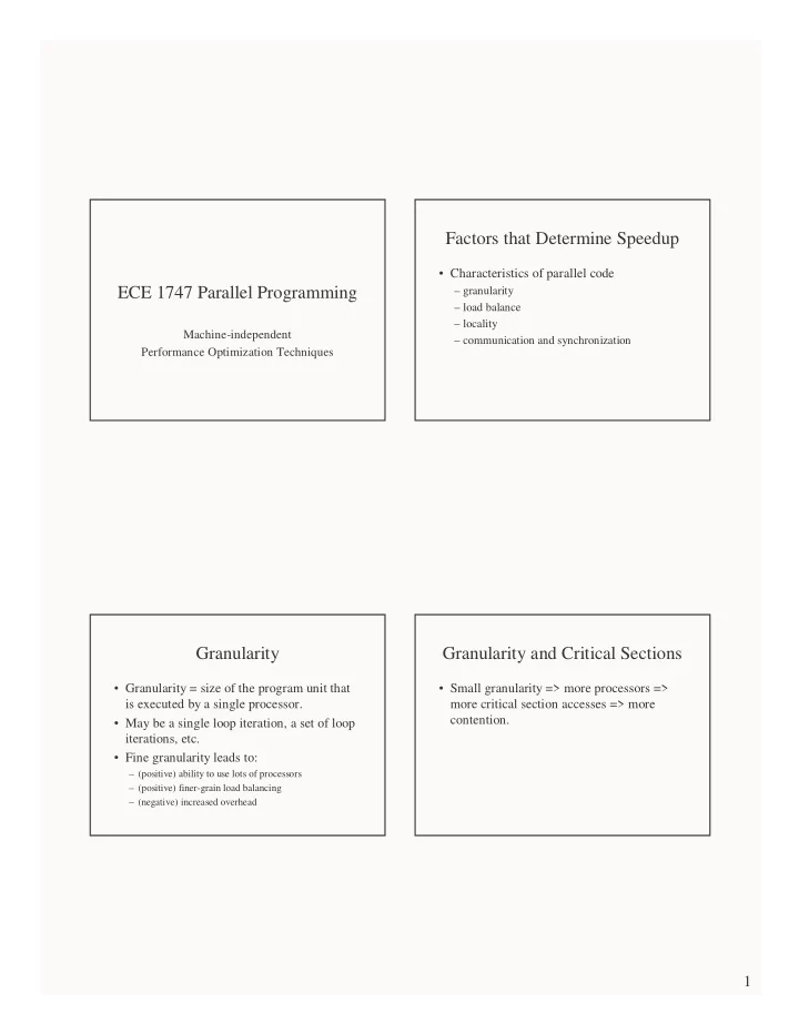
Factors that Determine Speedup • Characteristics of parallel code ECE 1747 Parallel Programming – granularity – load balance – locality Machine-independent – communication and synchronization Performance Optimization Techniques Granularity Granularity and Critical Sections • Granularity = size of the program unit that • Small granularity => more processors => is executed by a single processor. more critical section accesses => more contention. • May be a single loop iteration, a set of loop iterations, etc. • Fine granularity leads to: – (positive) ability to use lots of processors – (positive) finer-grain load balancing – (negative) increased overhead 1

Load Balance Issues in Performance of Parallel Parts • Load imbalance = different in execution • Granularity. time between processors between barriers. • Load balance. • Execution time may not be predictable. • Locality. – Regular data parallel: yes. • Synchronization and communication. – Irregular data parallel or pipeline: perhaps. – Task queue: no. Static vs. Dynamic Choice is not inherent • Static: done once, by the programmer • MM or SOR could be done using task – block, cyclic, etc. queues: put all iterations in a queue. – fine for regular data parallel – In heterogeneous environment. • Dynamic: done at runtime – In multitasked environment. – task queue • TSP could be done using static partitioning: – fine for unpredictable execution times – If we did exhaustive search. – usually high overhead • Semi-static: done once, at run-time 2

Static Load Balancing Dynamic Load Balancing (1 of 2) • Block • Centralized: single task queue. – best locality – Easy to program – possibly poor load balance – Excellent load balance • Cyclic • Distributed: task queue per processor. – better load balance – worse locality – Less communication/synchronization • Block-cyclic – load balancing advantages of cyclic (mostly) – better locality (see later) Dynamic Load Balancing (2 of 2) Semi-static Load Balancing • Task stealing: • Measure the cost of program parts. – Processes normally remove and insert tasks • Use measurement to partition computation. from their own queue. • Done once, done every iteration, done every – When queue is empty, remove task(s) from n iterations. other queues. • Extra overhead and programming difficulty. • Better load balancing. 3

Molecular Dynamics (continued) Molecular Dynamics (continued) for some number of timesteps { for each molecule i for all molecules i number of nearby molecules count[i] for all nearby molecules j array of indices of nearby molecules index[j] force[i] += f( loc[i], loc[j] ); ( 0 <= j < count[i]) for all molecules i loc[i] = g( loc[i], force[i] ); } Molecular Dynamics (continued) Molecular Dynamics (simple) for some number of timesteps { for some number of timesteps { Fork() for( i=0; i<num_mol; i++ ) for( i=0; i<num_mol; i++ ) for( j=0; j<count[i]; j++ ) for( j=0; j<count[i]; j++ ) force[i] += f(loc[i],loc[index[j]]); force[i] += f(loc[i],loc[index[j]]); Join() for( i=0; i<num_mol; i++ ) Fork() loc[i] = g( loc[i], force[i] ); for( i=0; i<num_mol; i++ ) } loc[i] = g( loc[i], force[i] ); } Join() 4

Molecular Dynamics (simple) Molecular Dynamics (simple) for some number of timesteps { • Simple to program. Parallel for • Possibly poor load balance for( i=0; i<num_mol; i++ ) – block distribution of i iterations (molecules) for( j=0; j<count[i]; j++ ) – could lead to uneven neighbor distribution force[i] += f(loc[i],loc[index[j]]); – cyclic does not help Parallel for for( i=0; i<num_mol; i++ ) loc[i] = g( loc[i], force[i] ); } Better Load Balance Molecular Dynamics (continued) for some number of timesteps { • Assign iterations such that each processor Parallel for has ~ the same number of neighbors. pr = get_thread_num(); • Array of “assign records” for( i=assign[pr]->b; i<assign[pr]->e; i++ ) – size: number of processors for( j=0; j<count[i]; j++ ) – two elements: force[i] += f(loc[i],loc[index[j]]); • beginning i value (molecule) Parallel for • ending i value (molecule) for( i=0; i<num_mol; i++ ) • Recompute partition periodically loc[i] = g( loc[i], force[i] ); } 5

Frequency of Balancing Summary • Every time neighbor list is recomputed. • Parallel code optimization – once during initialization. – Critical section accesses. – every iteration. – Granularity. – every n iterations. – Load balance. • Extra overhead vs. better approximation and better load balance. Factors that Determine Speedup Uniprocessor Memory Hierarchy size access time – granularity – load balancing memory – locality • uniprocessor • multiprocessor L2 cache – synchronization and communication L1 cache CPU 6

Typical Cache Organization Cache Replacement • Caches are organized in “cache lines”. • If you hit in the cache, done. • Typical line sizes • If you miss in the cache, – L1: 32 bytes – Fetch line from next level in hierarchy. – L2: 128 bytes – Replace a line from the cache. Bottom Line Locality • To get good performance, • Locality (or re-use) = the extent to which a processor continues to use the same data or – You have to have a high hit rate. “close” data. – You have to continue to access the data “close” to the data that you accessed recently. • Temporal locality: re-accessing a particular word before it gets replaced • Spatial locality: accessing other words in a cache line before the line gets replaced 7

Example 1 Example 2 for( i=0; i<n; i++ ) for( j=0; j<n; j++ ) for( j=0; j<n; j++ ) for( i=0; i<n; i++ ) grid[i][j] = temp[i][j]; grid[i][j] = temp[i][j]; • No spatial locality in grid and temp. • Good spatial locality in grid and temp (arrays in C laid out in row-major order). • No temporal locality. • No temporal locality. Example 3 Access to grid[i][j] for( i=0; i<n; i++ ) • First time grid[i][j] is used: temp[i-1,j]. for( j=0; j<n; j++ ) • Second time grid[i][j] is used: temp[i,j-1]. temp[i][j] = 0.25 * (grid[i+1][j]+grid[i+1][j]+ • Between those times, 3 rows go through the grid[i][j-1]+grid[i][j+1]); cache. • If 3 rows > cache size, cache miss on • Spatial locality in temp. second access for grid[i][j]. • Spatial locality in grid. • Temporal locality in grid? 8

Fix Example 3 (before) • Traverse the array in blocks, rather than row-wise sweep. • Make sure grid[i][j] still in cache on second access. Example 3 (afterwards) Achieving Better Locality • Technique is known as blocking / tiling. • Compiler algorithms known. • Few commercial compilers do it. • Learn to do it yourself. 9

Locality in Parallel Programming Returning to Sequential vs. Parallel • Is even more important than in sequential • A piece of code may be better executed programming, because the memory sequentially if considered by itself. latencies are longer. • But locality may make it profitable to execute it in parallel. • Typically happens with initializations. Example: Parallelization Ignoring Locality Example: Taking Locality into Account for( i=0; i<n; i++ ) Parallel for a[i] = i; for( i=0; i<n; i++ ) Parallel for a[i] = i; for( i=0; i<n; i++ ) Parallel for /* assume f is a very expensive function */ for( i=0; i<n; i++ ) b[i] = f( a[i-1], a[i] ); /* assume f is a very expensive function */ b[i] = f( a[i-1], a[i] ) 10

How to Get Started? Performance and Architecture • First thing: figure what takes the time in your • Understanding the performance of a parallel sequential program => profile it (gprof) ! program often requires an understanding of • Typically, few parts (few loops) take the bulk of the underlying architecture. the time. • There are two principal architectures: • Parallelize those parts first, worrying about granularity and load balance. – distributed memory machines • Advantage of shared memory: you can do that – shared memory machines incrementally. • Microarchitecture plays a role too! • Then worry about locality. 11