
SLIDE 1
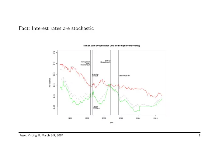
Fact: Interest rates are stochastic
1996 1998 2000 2002 2004 2006 0.02 0.04 0.06 0.08 0.10 0.12
Danish zero coupon rates (and some significant events)
year interest rate 0Y 30Y 15Y 5Y Amsterdam Treaty Referendum Russian default LTCM collapse EURO Referendum September 11
Asset Pricing II, March 8-9, 2007 1