... . . . 3. Uniform Probability Space: Pr [ ] = 1 / | | for all - - PowerPoint PPT Presentation

Continuing Probability.

Wrap up: Probability Formalism. Events, Conditional Probability, Independence, Bayes’ Rule

Probability Space: Formalism

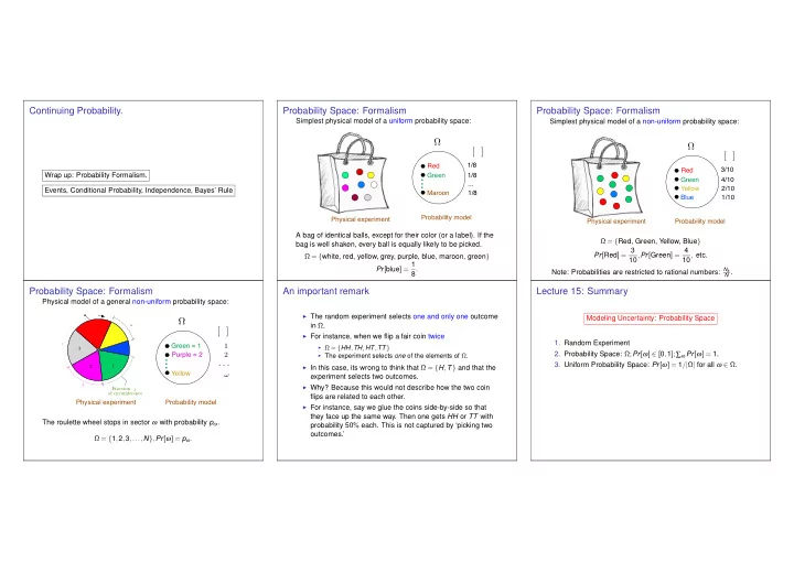
Simplest physical model of a uniform probability space:

Red Green Maroon

Ω

1/8 1/8 ... 1/8

P r [ω ]

. . .

Physical experiment Probability model

A bag of identical balls, except for their color (or a label). If the bag is well shaken, every ball is equally likely to be picked. Ω = {white, red, yellow, grey, purple, blue, maroon, green} Pr[blue] = 1 8.

Probability Space: Formalism

Simplest physical model of a non-uniform probability space:

Red Green Yellow Blue

Ω

3/10 4/10 2/10 1/10

P r [ω ]

Physical experiment Probability model

Ω = {Red, Green, Yellow, Blue} Pr[Red] = 3 10,Pr[Green] = 4 10, etc. Note: Probabilities are restricted to rational numbers: Nk

N .

Probability Space: Formalism

Physical model of a general non-uniform probability space:

p 3 Fraction p 1

• f circumference

p 2 p ω ω

1 2 3

Physical experiment Probability model Purple = 2 Green = 1 Yellow

Ω P r [ω ]

...

p 1 p 2 p ω . . . ω

The roulette wheel stops in sector ω with probability pω. Ω = {1,2,3,...,N},Pr[ω] = pω.

An important remark

◮ The random experiment selects one and only one outcome

in Ω.

◮ For instance, when we flip a fair coin twice

◮ Ω = {HH,TH,HT,TT} ◮ The experiment selects one of the elements of Ω.

◮ In this case, its wrong to think that Ω = {H,T} and that the

experiment selects two outcomes.

◮ Why? Because this would not describe how the two coin

flips are related to each other.

◮ For instance, say we glue the coins side-by-side so that

they face up the same way. Then one gets HH or TT with probability 50% each. This is not captured by ‘picking two

• utcomes.’

Lecture 15: Summary

Modeling Uncertainty: Probability Space

• 1. Random Experiment
• 2. Probability Space: Ω;Pr[ω] ∈ [0,1];∑ω Pr[ω] = 1.
• 3. Uniform Probability Space: Pr[ω] = 1/|Ω| for all ω ∈ Ω.

CS70: On to Calculation.

Events, Conditional Probability, Independence, Bayes’ Rule

• 1. Probability Basics Review
• 2. Events
• 3. Conditional Probability
• 4. Independence of Events
• 5. Bayes’ Rule

Probability Basics Review

Setup:

◮ Random Experiment.

Flip a fair coin twice.

◮ Probability Space.

◮ Sample Space: Set of outcomes, Ω.

Ω = {HH,HT,TH,TT} (Note: Not Ω = {H,T} with two picks!)

◮ Probability: Pr[ω] for all ω ∈ Ω.

Pr[HH] = ··· = Pr[TT] = 1/4

• 1. 0 ≤ Pr[ω] ≤ 1.
• 2. ∑ω∈Ω Pr[ω] = 1.

Set notation review

A B Ω

Figure: Two events

Ω ¯ A

Figure: Complement (not)

Ω A [ B

Figure: Union (or)

Ω A ∩ B

Figure: Intersection (and)

Ω A \ B

Figure: Difference (A, not B)

Ω A ∆B

Figure: Symmetric difference (only one)

Probability of exactly one ‘heads’ in two coin flips?

Idea: Sum the probabilities of all the different outcomes that have exactly one ‘heads’: HT,TH. This leads to a definition! Definition:

◮ An event, E, is a subset of outcomes: E ⊂ Ω. ◮ The probability of E is defined as Pr[E] = ∑ω∈E Pr[ω].

Event: Example

Red Green Yellow Blue

Ω

3/10 4/10 2/10 1/10

P r [ω ]

Physical experiment Probability model

Ω = {Red, Green, Yellow, Blue} Pr[Red] = 3 10,Pr[Green] = 4 10, etc. E = {Red,Green} ⇒ Pr[E] = 3+4 10 = 3 10 + 4 10 = Pr[Red]+Pr[Green].

Probability of exactly one heads in two coin flips?

Sample Space, Ω = {HH,HT,TH,TT}. Uniform probability space: Pr[HH] = Pr[HT] = Pr[TH] = Pr[TT] = 1

4.

Event, E, “exactly one heads”: {TH,HT}. Pr[E] = ∑

ω∈E

Pr[ω] = |E| |Ω| = 2 4 = 1 2.

Example: 20 coin tosses.

20 coin tosses

Sample space: Ω = set of 20 fair coin tosses. Ω = {T,H}20 ≡ {0,1}20; |Ω| = 220.

◮ What is more likely?

◮ ω1 := (1,1,1,1,1,1,1,1,1,1,1,1,1,1,1,1,1,1,1,1), or ◮ ω2 := (1,0,1,1,0,0,0,1,0,1,0,1,1,0,1,1,1,0,0,0)?

Answer: Both are equally likely: Pr[ω1] = Pr[ω2] =

1 |Ω|. ◮ What is more likely?

(E1) Twenty Hs out of twenty, or (E2) Ten Hs out of twenty?

Answer: Ten Hs out of twenty. Why? There are many sequences of 20 tosses with ten Hs;

• nly one with twenty Hs. ⇒ Pr[E1] =

1 |Ω| ≪ Pr[E2] = |E2| |Ω| .

|E2| = 20 10

• = 184,756.

Probability of n heads in 100 coin tosses.

Ω = {H,T}100; |Ω| = 2100.

n p n

Event En = ‘n heads’; |En| = 100

n

• pn := Pr[En] = |En|

|Ω| = (100

n )

2100

Observe:

◮ Concentration around mean:

Law of Large Numbers;

◮ Bell-shape: Central Limit

Theorem.

Roll a red and a blue die. Exactly 50 heads in 100 coin tosses.

Sample space: Ω = set of 100 coin tosses = {H,T}100. |Ω| = 2×2×···×2 = 2100. Uniform probability space: Pr[ω] =

1 2100 .

Event E = “100 coin tosses with exactly 50 heads” |E|? Choose 50 positions out of 100 to be heads. |E| = 100

50

• .

Pr[E] = 100

50

• 2100 .

Calculation. Stirling formula (for large n): n! ≈ √ 2πn n e n . 2n n

• ≈

√ 4πn(2n/e)2n [ √ 2πn(n/e)n]2 ≈ 4n √πn. Pr[E] = |E| |Ω| = |E| 22n = 1 √πn = 1 √ 50π ≈ .08.

Exactly 50 heads in 100 coin tosses.

Probability is Additive

Theorem (a) If events A and B are disjoint, i.e., A∩B = / 0, then Pr[A∪B] = Pr[A]+Pr[B]. (b) If events A1,...,An are pairwise disjoint, i.e., Ak ∩Am = / 0,∀k = m, then Pr[A1 ∪···∪An] = Pr[A1]+···+Pr[An]. Proof:

Obvious.

Consequences of Additivity

Theorem (a) Pr[A∪B] = Pr[A]+Pr[B]−Pr[A∩B]; (inclusion-exclusion property) (b) Pr[A1 ∪···∪An] ≤ Pr[A1]+···+Pr[An]; (union bound) (c) If A1,...AN are a partition of Ω, i.e., pairwise disjoint and ∪N

m=1Am = Ω, then

Pr[B] = Pr[B ∩A1]+···+Pr[B ∩AN]. (law of total probability) Proof: (b) is obvious. Proofs for (a) and (c)? Next...

Inclusion/Exclusion

Pr[A∪B] = Pr[A]+Pr[B]−Pr[A∩B] Another view. Any ω ∈ A∪B is in A∩B, A∪B, or A∩B. So, add it up.

Total probability

Assume that Ω is the union of the disjoint sets A1,...,AN. Then, Pr[B] = Pr[A1 ∩B]+···+Pr[AN ∩B]. Indeed, B is the union of the disjoint sets An ∩B for n = 1,...,N. In “math”: ω ∈ B is in exactly one of Ai ∩B. Adding up probability of them, get Pr[ω] in sum. ..Did I say... Add it up.

Roll a Red and a Blue Die.

E1 = ‘Red die shows 6’;E2 = ‘Blue die shows 6’ E1 ∪E2 = ‘At least one die shows 6’ Pr[E1] = 6 36,Pr[E2] = 6 36,Pr[E1 ∪E2] = 11 36.

Conditional probability: example.

Two coin flips. First flip is heads. Probability of two heads? Ω = {HH,HT,TH,TT}; Uniform probability space. Event A = first flip is heads: A = {HH,HT}. New sample space: A; uniform still. Event B = two heads. The probability of two heads if the first flip is heads. The probability of B given A is 1/2.

A similar example.

Two coin flips. At least one of the flips is heads. → Probability of two heads? Ω = {HH,HT,TH,TT}; uniform. Event A = at least one flip is heads. A = {HH,HT,TH}. New sample space: A; uniform still. Event B = two heads. The probability of two heads if at least one flip is heads. The probability of B given A is 1/3.

Conditional Probability: A non-uniform example

Red Green Yellow Blue

Ω

3/10 4/10 2/10 1/10

P r [ω ]

Physical experiment Probability model

Ω = {Red, Green, Yellow, Blue} Pr[Red|Red or Green] = 3 7 = Pr[Red∩(Red or Green)] Pr[Red or Green]

Another non-uniform example

Consider Ω = {1,2,...,N} with Pr[n] = pn. Let A = {3,4},B = {1,2,3}. Pr[A|B] = p3 p1 +p2 +p3 = Pr[A∩B] Pr[B] .

Yet another non-uniform example

Consider Ω = {1,2,...,N} with Pr[n] = pn. Let A = {2,3,4},B = {1,2,3}. Pr[A|B] = p2 +p3 p1 +p2 +p3 = Pr[A∩B] Pr[B] .

Conditional Probability.

Definition: The conditional probability of B given A is Pr[B|A] = Pr[A∩B] Pr[A] A B A B In A! In B? Must be in A∩B. A∩B Pr[B|A] = Pr[A∩B]

Pr[A] .

More fun with conditional probability.

Toss a red and a blue die, sum is 4, What is probability that red is 1? Pr[B|A] = |B∩A|

|A|

= 1

3; versus Pr[B] = 1/6.

B is more likely given A.

Yet more fun with conditional probability.

Toss a red and a blue die, sum is 7, what is probability that red is 1? Pr[B|A] = |B∩A|

|A|

= 1

6; versus Pr[B] = 1 6.

Observing A does not change your mind about the likelihood of B.

Emptiness..

Suppose I toss 3 balls into 3 bins. A =“1st bin empty”; B =“2nd bin empty.” What is Pr[A|B]? Pr[B] = Pr[{(a,b,c) | a,b,c ∈ {1,3}] = Pr[{1,3}3] = 8

27

Pr[A∩B] = Pr[(3,3,3)] = 1

27

Pr[A|B] = Pr[A∩B]

Pr[B]

= (1/27)

(8/27) = 1/8; vs. Pr[A] = 8 27.

A is less likely given B: If second bin is empty the first is more likely to have balls in it.

Three Card Problem

Three cards: Red/Red, Red/Black, Black/Black. Pick one at random and place on the table. The upturned side is a

• Red. What is the probability that the other side is Black?

Can’t be the BB card, so...prob should be 0.5, right? R: upturned card is Red; RB: the Red/Black card was selected. Want P(RB|R). What’s wrong with the reasoning that leads to 1

2?

P(RB|R) = P(RB ∩ R) P(R) =

1 3 1 2 1 3(1) + 1 3 1 2 + 1 3(0)

=

1 6 1 2

= 1 3 Once you are given R: it is twice as likely that the RR card was picked.

4

Gambler’s fallacy.

Flip a fair coin 51 times. A = “first 50 flips are heads” B = “the 51st is heads” Pr[B|A] ? A = {HH ···HT,HH ···HH} B ∩A = {HH ···HH} Uniform probability space. Pr[B|A] = |B∩A|

|A|

= 1

2.

Same as Pr[B].

The likelihood of 51st heads does not depend on the previous flips.

Product Rule

Recall the definition: Pr[B|A] = Pr[A∩B] Pr[A] . Hence, Pr[A∩B] = Pr[A]Pr[B|A]. Consequently, Pr[A∩B ∩C] = Pr[(A∩B)∩C] = Pr[A∩B]Pr[C|A∩B] = Pr[A]Pr[B|A]Pr[C|A∩B].

Product Rule

Theorem Product Rule Let A1,A2,...,An be events. Then Pr[A1 ∩···∩An] = Pr[A1]Pr[A2|A1]···Pr[An|A1 ∩···∩An−1]. Proof: By induction. Assume the result is true for n. (It holds for n = 2.) Then,

Pr[A1 ∩···∩An ∩An+1] = Pr[A1 ∩···∩An]Pr[An+1|A1 ∩···∩An] = Pr[A1]Pr[A2|A1]···Pr[An|A1 ∩···∩An−1]Pr[An+1|A1 ∩···∩An],

so that the result holds for n +1.

Correlation

An example. Random experiment: Pick a person at random. Event A: the person has lung cancer. Event B: the person is a heavy smoker. Fact: Pr[A|B] = 1.17×Pr[A]. Conclusion:

◮ Smoking increases the probability of lung cancer by 17%. ◮ Smoking causes lung cancer.

Correlation

Event A: the person has lung cancer. Event B: the person is a heavy smoker. Pr[A|B] = 1.17×Pr[A]. A second look. Note that Pr[A|B] = 1.17×Pr[A] ⇔ Pr[A∩B] Pr[B] = 1.17×Pr[A] ⇔ Pr[A∩B] = 1.17×Pr[A]Pr[B] ⇔ Pr[B|A] = 1.17×Pr[B]. Conclusion:

◮ Lung cancer increases the probability of smoking by 17%. ◮ Lung cancer causes smoking. Really?

Causality vs. Correlation

Events A and B are positively correlated if Pr[A∩B] > Pr[A]Pr[B]. (E.g., smoking and lung cancer.) A and B being positively correlated does not mean that A causes B or that B causes A. Other examples:

◮ Tesla owners are more likely to be rich. That does not

mean that poor people should buy a Tesla to get rich.

◮ People who go to the opera are more likely to have a good

• career. That does not mean that going to the opera will

improve your career.

◮ Rabbits eat more carrots and do not wear glasses. Are

carrots good for eyesight?

Total probability

Assume that Ω is the union of the disjoint sets A1,...,AN. Then, Pr[B] = Pr[A1 ∩B]+···+Pr[AN ∩B]. Indeed, B is the union of the disjoint sets An ∩B for n = 1,...,N. Thus, Pr[B] = Pr[A1]Pr[B|A1]+···+Pr[AN]Pr[B|AN].

Total probability

Assume that Ω is the union of the disjoint sets A1,...,AN. Pr[B] = Pr[A1]Pr[B|A1]+···+Pr[AN]Pr[B|AN].

Is your coin loaded?

Your coin is fair w.p. 1/2 or such that Pr[H] = 0.6, otherwise. You flip your coin and it yields heads. What is the probability that it is fair? Analysis: A = ‘coin is fair’,B = ‘outcome is heads’ We want to calculate P[A|B]. We know P[B|A] = 1/2,P[B|¯ A] = 0.6,Pr[A] = 1/2 = Pr[¯ A] Now, Pr[B] = Pr[A∩B]+Pr[¯ A∩B] = Pr[A]Pr[B|A]+Pr[¯ A]Pr[B|¯ A] = (1/2)(1/2)+(1/2)0.6 = 0.55. Thus, Pr[A|B] = Pr[A]Pr[B|A] Pr[B] = (1/2)(1/2) (1/2)(1/2)+(1/2)0.6 ≈ 0.45.

Is your coin loaded?

A picture: Imagine 100 situations, among which m := 100(1/2)(1/2) are such that A and B occur and n := 100(1/2)(0.6) are such that ¯ A and B occur. Thus, among the m +n situations where B occurred, there are m where A occurred. Hence, Pr[A|B] = m m +n = (1/2)(1/2) (1/2)(1/2)+(1/2)0.6.

Independence

Definition: Two events A and B are independent if Pr[A∩B] = Pr[A]Pr[B]. Examples:

◮ When rolling two dice, A = sum is 7 and B = red die is 1

are independent;

◮ When rolling two dice, A = sum is 3 and B = red die is 1

are not independent;

◮ When flipping coins, A = coin 1 yields heads and B = coin

2 yields tails are independent;

◮ When throwing 3 balls into 3 bins, A = bin 1 is empty and

B = bin 2 is empty are not independent;

Independence and conditional probability

Fact: Two events A and B are independent if and only if Pr[A|B] = Pr[A]. Indeed: Pr[A|B] = Pr[A∩B]

Pr[B] , so that

Pr[A|B] = Pr[A] ⇔ Pr[A∩B] Pr[B] = Pr[A] ⇔ Pr[A∩B] = Pr[A]Pr[B].

Bayes Rule

Another picture: We imagine that there are N possible causes A1,...,AN. Imagine 100 situations, among which 100pnqn are such that An and B occur, for n = 1,...,N. Thus, among the 100∑m pmqm situations where B occurred, there are 100pnqn where An occurred. Hence, Pr[An|B] = pnqn ∑m pmqm .

Why do you have a fever?

Using Bayes’ rule, we find Pr[Flu|High Fever] = 0.15×0.80 0.15×0.80+10−8 ×1+0.85×0.1 ≈ 0.58 Pr[Ebola|High Fever] = 10−8 ×1 0.15×0.80+10−8 ×1+0.85×0.1 ≈ 5×10−8 Pr[Other|High Fever] = 0.85×0.1 0.15×0.80+10−8 ×1+0.85×0.1 ≈ 0.42 These are the posterior probabilities. One says that ‘Flu’ is the Most Likely a Posteriori (MAP) cause of the high fever.

Bayes’ Rule Operations

Bayes’ Rule is the canonical example of how information changes our opinions.

Thomas Bayes

Source: Wikipedia.

Thomas Bayes

A Bayesian picture of Thomas Bayes.

Testing for disease.

Let’s watch TV!! Random Experiment: Pick a random male. Outcomes: (test,disease) A - prostate cancer. B - positive PSA test.

◮ Pr[A] = 0.0016, (.16 % of the male population is affected.) ◮ Pr[B|A] = 0.80 (80% chance of positive test with disease.) ◮ Pr[B|A] = 0.10 (10% chance of positive test without

disease.) From http://www.cpcn.org/01 psa tests.htm and http://seer.cancer.gov/statfacts/html/prost.html (10/12/2011.) Positive PSA test (B). Do I have disease? Pr[A|B]???

Bayes Rule.

Using Bayes’ rule, we find P[A|B] = 0.0016×0.80 0.0016×0.80+0.9984×0.10 = .013. A 1.3% chance of prostate cancer with a positive PSA test. Surgery anyone? Impotence... Incontinence.. Death.

Summary

Events, Conditional Probability, Independence, Bayes’ Rule Key Ideas:

◮ Conditional Probability:

Pr[A|B] = Pr[A∩B]

Pr[B] ◮ Independence: Pr[A∩B] = Pr[A]Pr[B]. ◮ Bayes’ Rule:

Pr[An|B] = Pr[An]Pr[B|An] ∑m Pr[Am]Pr[B|Am]. Pr[An|B] = posterior probability;Pr[An] = prior probability .

◮ All these are possible:

Pr[A|B] < Pr[A];Pr[A|B] > Pr[A];Pr[A|B] = Pr[A].